Electrostatic Laws: were deduced in the 1700's by experiments with macroscopic charged bodies. Coulomb's experiments on the forces between charged spheres led to the Coulomb inverse-square law for the force between two charged particles. With the introduction of the idea of a "field," came the notion that this force derives from the influence of the electrostatic field (E) of one particle acting upon the other.
Magnetostatic Laws: In 1819 Oersted noticed that an electric current flowing in a wire deflected a nearby compass. Soon after Biot and Savart quantified the magnetic field due to steady current in a long straight wire. Ampere found that two current-carrying wires interacted by magnetic forces; and postulated that all magnetic fields have their origin in electrical currents, at the macroscopic or microscopic level. Faraday (1830's) observed a current was induced to flow in a closed circuit when a nearby magnet was moved, or the current in a nearby circuit was changed, or the test circuit was moved in a steady magnetic field.
Unification: Maxwell in the 1860's assembled various known results describing static and dynamic electric and magnetic forces into a general framework of time-dependent differential eqns. These equations had wave solutions, and the speed of the waves turned out to match the (already known) speed of light - leading Maxwell to the realisation that light is an electromagnetic phenomenon. This was a great accomplishment - to have unified diverse phenomena.
Unification completed: Einstein (ealy 1900's) realized that Maxwell's equations for electro-magnetism were "covariant" with respect to the coordinate transformation (Lorenz transformation) of special relativity, ie. that these equations hold (unchanged) for all observers in uniform (unaccelerated) motion. The laws of transformation of electric and magnetic fields were given, showing that a pure electric field in one reference frame may entail both electric and magnetic fields in another, and vice versa.
Across the history of science, there have been alternating phases of belief that "light" consists of particles, and that (alternatively) light "is" a "wave" (a postulate that is required to explain interference and diffraction; it was until early this century believed the light-wave propogated on some "medium" that "waved," the ether).
Since the advent of quantum mechnics, we have arrived at the uncomfortable vagueness of accepting that light (more generally, E/M radiation) has a dual nature. In some experiments, light seems to behave as if streaming in particles (quanta) called "photons," while in other experiments the wave nature of light is pre-eminent.
The speed (c), wavelength (λ) and frequency (ν) of light are connected according to:
c=ν λ.
The energy carried by a photon is related to the wavelength of the corresponding wave
E = h ν
where the proportionality constant h is Planck's constant.
E/M radiation is generated by the acceleration of charge (a radio aerial is simply a conductor in which electrons are accelerated first one way, then back). All matter whose temperature is above absolute zero (0 K) emits radiation. For a particular (ideal) type of surface, namely the "black body," the rate (Φ) of energy emission per unit surface area of emitter is maximal (for the given temperature), and given by the (originally empirical) Stefan-Boltzmann Law
Φ [J m-2 s-1] = σ T4
where σ=5.67 x 10⁻⁸ [W m-2 K-4] is the Stefan-Boltzmann constant. A "black body" is defined to be a body that absorbs any photon that falls upon it (absorptivity = 1) and is the most efficient of all possible emitters. A "black body cavity" is an isothermal chamber, into a wall of which a tiny hole (area A) is drilled. Such an apparatus closely approximates an ideal black body...
Photons are classified as being of solar origin ("short wave") if their wavelength λ is in the range 0.3 to 4 μm, and of terrestrial origin ("long wave") if their wavelength is in the range 4 to 80 μm. Correspondingly, radiometers are classified as being short wave, long wave, or all-wave devices.
2. Definition of "Intensity" of radiative transfer in a given waveband
Radiative transfer is omnidirectional (photons can fly in any direction). The basic descriptor of the radiation field is the spectral intensity
I(x,s,λ) [J s-1 m-2 steradian-1 μm-1]
defined to be the intensity of energy transfer in waveband λ -> λ + d λ at position x into a cone of unit solid angle about the direction denoted by the unit vector s.
3. Transducer Principle
There are essentially two types of sensor used in radiometers.
Photovoltaic
A semiconductor produces a voltage which depends on the incident energy flux in all wavebands, but is generally not equally sensitive within all wavebands. Symbolically,
V = Σi αi dQi dλ
Here Σi means "sum over all bands (i)." The sum is made up of products: dQi is the energy flux density incident in the ith waveband divided by the width (dλ) of the waveband [the units of dQi are typically W m-2 μm-1]; and αi is the sensitivity of the transducer with the ith waveband. In the above formula all wavebands have equal width, dλ.
The major problem with photovoltaic transducers in the meteorological context is that, they do not have a sensitivity which is independent of wavelength, ie. they are selective in their response: whereas the radiometers outlined above need a sensor which is uniformly reponsive within the short wave, long wave, or allwave (entire) spectrum.
Thermometric
In this class of sensor the incident radiant flux(es) induce a temperature gradient within the device which is detected, usually by a thermopile, to produce an output. A major drawback of such a device is that the temperature distribution within a body immersed in the atmosphere is a complex function of the device energy balance, sensitive to geometry, convective exchanges, internal conduction, even latent heat exchange if the body is wet. These problems are overcome by careful design.
4. The net radiometer
Because of its importance, we will study the Net Radiometer in detail, as an example of the thermometric class of devices.
Firstly, we note that black paint has low reflectivity in both the short wave band and the longwave - whereas white paint is highly reflective in the short wave, but not so in the longwave. Since for a net radiometer we want uniform spectral response (ie. the contributions from short and long wave photons arriving from the same direction must contribute to the temperature gradient we will sense in proportion only to the energy of the photon) we would be crazy to use white paint on the absorbing ("seeing") surface.
We will use a black paint (specialised paints are available). Nevertheless no surface will have a spectrally uniform absorptivity, ie. even with a specially chosen black paint, a given energy flux in the short wave may give a different thermal gradient within the radiometer from that caused by the same energy flux in the long wave. This type of error can be "tuned" out by the manufacturer by painting some small proportion of one or both sides white (this can be seen on some but not all net radiometers). In setting up a simple mathematical model of the Net Radiometer, we shall focus on the temperature difference across that part of the radiometer whose faces are the upward- and downward-facing absorbtive surfaces. Subscripts t,b denote the top and bottom surfaces. Recall that in the long wave band, the absorbtivity of a surface is equal to the "emissivity" (ε) of the surface.
The total downward energy flux is Qdn=Kdn+Ldn, so we may define an allwave absorptivity at for the top surface as
at Qdn = astKdn + εtLdn
where ast is the shortwave absorptivity for the top surface. It follows that
at = (astKdn+εtLdn)/(Kdn+Ldn)
which tells us that unless we can get both ast and εt unity we will have an overall absorbtivity at that depends upon Kdn and Ldn. A similar argument holds for ab.
Now we consider the energy balance of the top and bottom faces, bearing in mind that energy cannot accumulate at a plane: so that the sum of all the fluxes to and away from a plane must vanish. Assuming Qdn >0 (as it would be in sunlight), we have the top surface gaining energy from above radiatively, sending some back off through its own thermal radiation, shedding some by heat loss to the airstream (possibly), and conducting some away through the substrate. If h (= ρa cpa / rH ) is the "convective heat transfer coefficient," σ is the Stefan-Boltzmann constant ( σ =5.67 x 10⁻⁸ W m-2 K-4), and k is the thermal conductivity of the substrate, the energy balances of the two surfaces are:
at Qdn = εt σ Tt4 + h (Tt - Ta) + k (Tt-Tb)/d
ab Qup = εb σ Tb4 + h (Tb - Ta) - k (Tt-Tb)/d
Now lets assume εt=εb=ε, and at=ab=a. Subtracting the above formulae:
a (Qdn-Qup) = a Q* = ε σ (Tt4-Tb4) + h (Tt - Tb) +2 k (Tt-Tb)/d
We have a non-linear term in the radiometer temperatures, which we can simplify. All these temperatures should be in K and we know that Tt-Tb is small compared to Tt and Tb. So we make the approximation that
Tt4 ~ Tb4 + (dT4/dT)T=Tt (Tt - Tb) = Tb4 + 4 Tt3 (Tt - Tb)
With this approximation:
a Q* = (4ε σ Tt3 + 2k/d + h) (Tt - Tb).
Now suppose we put a dome over each side of the radiometer that is transparent to radiation, but drastically reduces convective heat loss. All going well, we thereby reduce h to zero: neither side loses heat convectively to the airstream.
Now some numbers. If the medium is aluminum, k=236 W m-1 K-1. If d=5 mm then 2k/d=9.4x104 whereas 4ε σ Tt3 is about 6. So our analysis suggests that
a Q* = (2k/d) (Tt - Tb).
A temperature gradient (Tt-Tb) arises in the medium, of a strength that is in linear proportion to the net radiation, the proportionality constant being independent of environmental factors, and dependent only on the design of the radiometer. Thus we have
Q* = C' (Tt-Tb) = C V
where C is the calibration coefficient, and V is the output voltage from the thermopile sensing (Tt-Tb). However note all the possible places our argument can go wrong.
A sensor for Qdn can be obtained by covering the lower side of a net radiometer with a heavy and isothermal cup, having a blackened interior, and known temperature Tcup. Then the apparent net radiation C V (where V is the output voltage) is given by:
C V = Qdn - σ Tcup4.
5. The Cosine response of a hemispherical radiometer.
Suppose a uniform beam of photons strikes a radiometer at normal incidence, and that, in that condition, the radiometer voltage signal is V=Vo. Now as we incline the absorbing surface of the radiometer away from the beam through angle θ , if the response is V=Vocos(θ) we have a perfect cosine response. Many radiometers deviate from ideal cosine response as θ approaches 90o; the surface reflectivity of the radiometer often increases for photons arriving at grazing incidence.
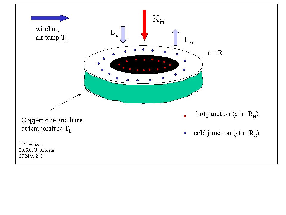
6. Hemispherical Solarimeter.
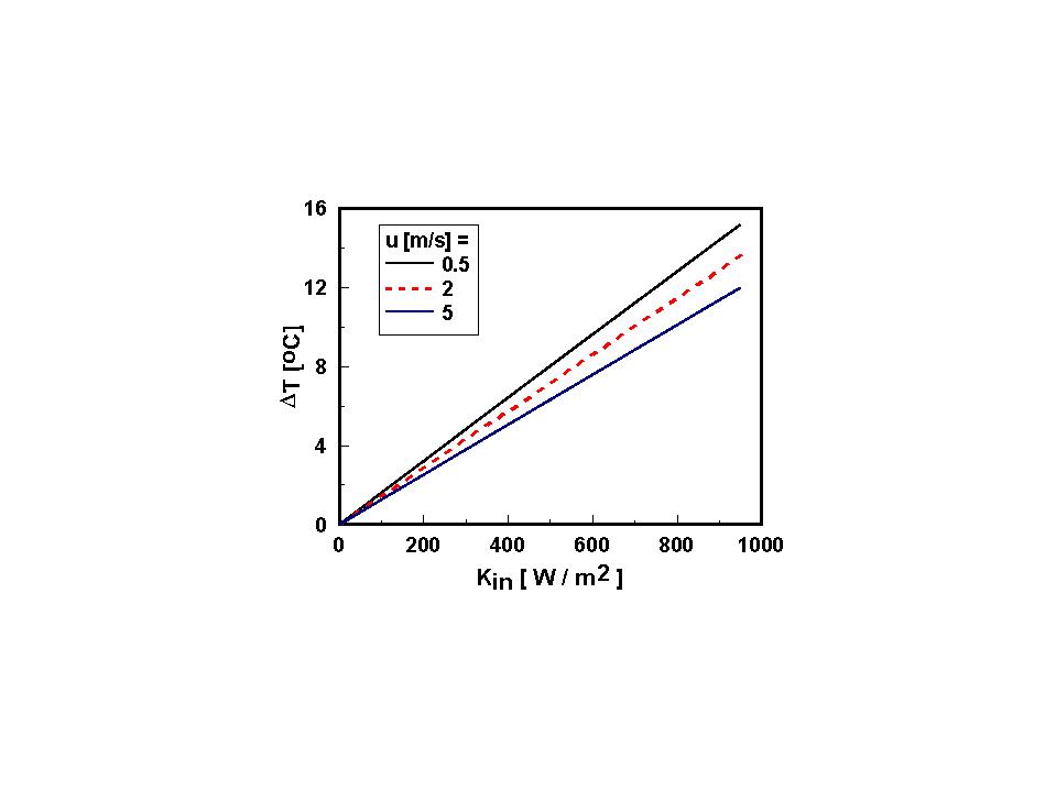
We will now study a simple model of a solarimeter. For now, consider that the device, a plexiglass disk with a painted upper surface, is fully exposed to the wind (no dome). The upper surface (z=0) has an inner region that is painted black, the remainder of the top surface being white. Solar insolation (Kin) will cause a temperature difference ΔT between the "hot junctions" (TH) and the "cold junctions" (TC) and this will be sensed by a thermopile.
In order to figure out whether the temperature difference ΔT has a meaningful relationship with Kin (which is what we want to measure), we have to figure out the temperature "field" in the plexiglass, T=T(t,r,z). The latter statement says, "T is a function of time and position, where position is measured in terms of radial distance r from the axis and depth z below the top surface)." To determine the field of T, we need to solve the "heat equation" with appropriate boundary and initial conditions. The "heat equation" is just the equation that expresses conservation of thermal energy within the volume of the device. If we content ourselves with a steady-state analysis, then the heat equation, expressed in a cylindrical coordinate system (radius r, depth z), is:
0 = (1/r) ∂/∂r (r k ∂T/∂r) + k ∂2T/∂z2
where k is the conductivity of the plexiglass. This is a 2nd-order partial differential equation. Basically this equation determines the temperature field within the volume of the sensor, based on the conditions imposed on the sides. We will need two of those "boundary conditions" on each axis. These are:
(- k ∂T/∂z)z=0 = Kin ( 1 - re(r)) + Lin - σ T(r)4 - ρa cpa ( T(r) - Ta) / rH
where re=re(r) is the local shortwave reflectivity (varying with r, ie. changing between the black and the white-painted surface); rH is the heat transfer resistance for the disc, a function of the disc dimensions and the windspeed (this can be prescribed by the usual route: find a Nu correlation). For simplicity, lets assume Lin = σ Ta4.
A numerical solution for the hot-cold temperature difference indicates a linear response to Kin. For this calculation values assumed for the device were: radius R=3cm; depth d= 2 cm; Ta=Tb=293 K; reflectivity step change at r=1 cm from re=0.9 to re=0.2; hot junction radius RH=0.2 cm; cold junction radius RC=2.5 cm.
The (unwanted) response to windspeed may be reduced by adding a dome.
7. IR Radiation thermometer.
The infra-red radiation thermometer is designed to remotely sense the temperature of a target surface, by virtue of the infra-red (ie., longwave) radiation it receives from the target. In the device illustrated, the radiation (wavelength λ) falls on a thermistor, whose resistance R is a function of its temperature Ts. That thermistor is one element of a Wheatstone bridge. A light chopper wheel alternately switches in and bars a flux of longwave radiation from outside, that flux being a function of IR emission in the field of view of the device, which is controlled by the optics (a lens). An optical filter selects the operating waveband. When the shutter is closed, the sensor sees radiation from within the walls of the isothermal cavity. In consequence, the error voltage of the Wheatstone bridge goes through a 100 Hz cycle, whose amplitude is related to the difference in temperature between the target, and the internal cavity. Internal electronics translate that signal into an output, giving the apparent target temperature. It is assumed that the emissivity of the target ε=1, and this is a potential source of error.
For example the Barnes PRT-5 device has a field of view of (nominally) 2o, and operates over the waveband 8-14 μm. It is claimed to be accurate to within 0.5oC, and to have a sensitivity ΔT that is better than 0.1oC.
Back to the Earth & Atmospheric Sciences home page.