1.0 Introductory Concepts
A variable x is discrete if it can take on only particular values (eg., if x can only take integer value, it is discrete). Contrariwise, we say x is continuous on range [a,b] if it can take on any value a <= x <= b.
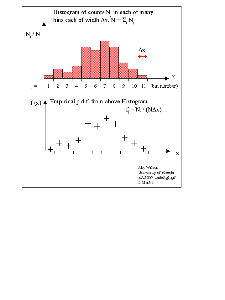
2.0 Histogram
Suppose we take a set of N observations (x1, x2, x3, ... xi, ...xN) of a random variable x (in standard shorthand notation, our sequence of observed values is denoted xi, i=1...N). And now suppose that we count the number Nj of these observations that fall into each of a number of ranges, or "bins," where the jth bin covers some range xj-min <= x <= xj-max and we say this bin has width Δxj = xj-max - xj-min. The ratios Nj/N <= 1 are the relative frequencies with which the random number x falls into bin j. If our sample is large enough, Nj/N should be a good estimator for the probability a single sample x falls into the jth bin. If we plot the Nj/N versus the centre-point values xj of the bins, we have the Histogram.
Now, let all the Δxj be equal (call this constant Δx) and define fj= 1/Δx Nj/N . We may plot fj against xj. All this does is to re-scale the Histogram, but this "f" is now an empirical (ie., observed) Probability Density Function (pdf) for the random variable x. The pdf of a random variable is an extremely important function, and from it, we may extract complete statistical knowledge of x. We'll begin for now by noting some crucial properties of the pdf.
f(x) = 1 / ((2π)½ σx) exp [ - (x - μ)2/ (2σx2)]
where μ is the population mean value of x, and σx is the population standard deviation. The "population" is the infinity of values of x we might have drawn - as distinct from a sample, which is drawn from the population. Note that the Gaussian distribution is a two-parameter distribution, and describes a random variable that has unrestricted range.
f(x) = α exp(-α x)
which evidently can only describe a "one-sided" variable, x >= 0. The single parameter α of the exponential distribution is related to both the mean and the standard deviation of the variable (see assigned problem).
3.0 Sample versus Population
So any given sample of N observations (x1, x2, x3, ... xi, ...xN) is finite. From it we can calculate properties called statistics, eg. the average value of x across the sample, denoted ⟨x⟩. This sample average can only be claimed to be an estimate of the average value (μ) of x across the population... so we say ⟨x⟩ is a statistic, while μ is a "parameter." And the usual reason for calculating statistics of a sample, is to estimate the parameters of the population.
4.0 Parameters, in particular "Moments," of a pdf.
The moments of a pdf f(x) are the "expected values" of x, of x2, of x3, and so forth. Many terminologies are used, and perhaps the best here is the E[ ] notation. Then, the expected value of x is denoted E[x], and this is the population mean, commonly given the symbol μ (as noted above, it is conventional to use Greek symbols to represent the parameters of a population, which are distinct from the statistics of a sample).
The rule for calculating the expected value of any variable g=g(x) that is a function of x, where x is a random variable defined on the range a <= x <= b, is very simple:
E[ g(x) ] = a∫b g(x) f(x) dx
It follows at once that the population mean is:
μ = E[x] = a∫b x f(x) dx
while
E[x2]= a∫b x2 f(x) dx
Higher "moments about the mean" are defined like (for example)
σ2 = a∫b (x-μ)2 f(x) dx
and this σ2 is nothing other than the population variance (= second moment about the mean), whose square root is the standard deviation.
5.0 Calculating Statistics of a Sample
From a sample of N observations (x1, x2, x3, ... xi, ...xN) we can calculate...
Sample Mean
mx = ⟨x⟩ = 1/N Σi xi
Sample Variance
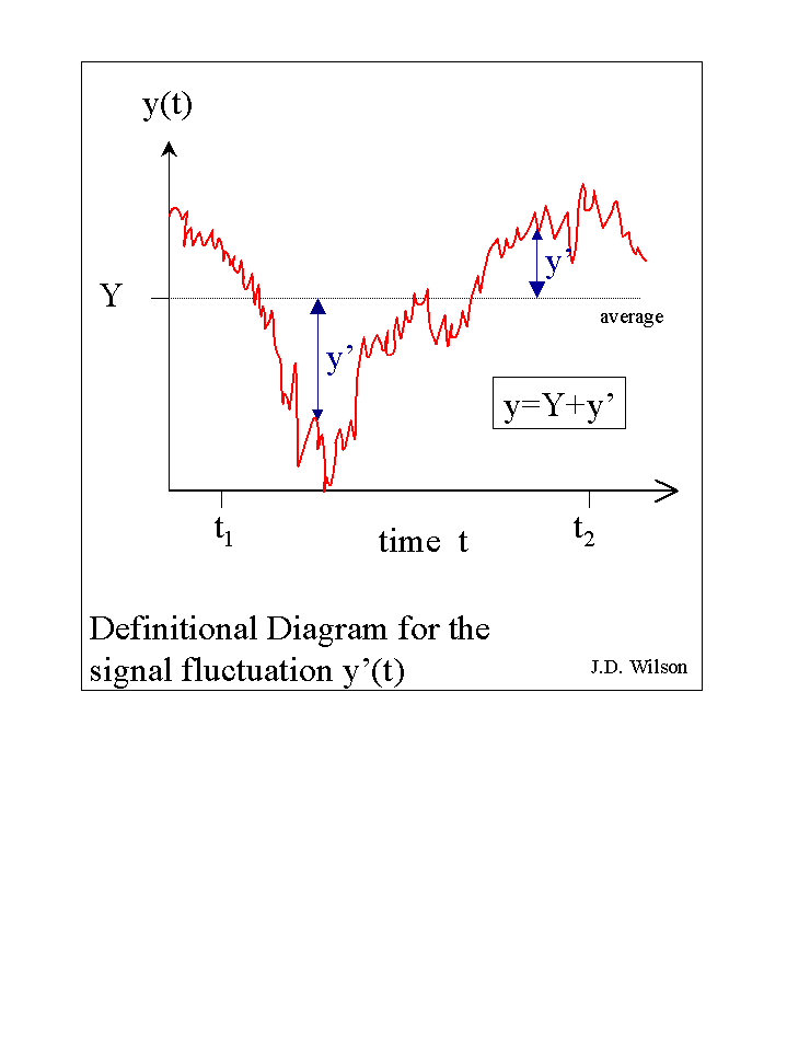
Define xi' = xi - ⟨x⟩ to be the deviation or fluctuation from the sample mean of the ith sample-member xi (the figure shows a random variable called "y", instead of x, a difference which is only a trivial matter of a name). Then we may calculate the sample variance sx2 (which is simply the square of the sample standard deviation sx) as:
sx2 = ⟨ x'2 ⟩ = ⟨ (x - ⟨x⟩)2 ⟩ = ⟨ x2 ⟩ - (⟨x⟩)2 =
= 1/N Σi x'i2 = 1/N Σi (xi - ⟨x⟩)2 = 1/N Σi xi2 - ( 1/N σi xi )2
where all these alternative forms are given to you to familiarise you with different notations (the first line) and different calculational procedures for obtaining the variance and standard deviation (the last three lines are alternative but equivalent recipes for calculation of the sample variance sx2). Of course the sample standard deviation is important as a measure of the spread of values xi observed in our sample.
The sample mean and standard deviation (mx, sx ; note the use of Roman rather than Greek symbols) are the two most common, important and familiar sample statistics, and are often considered without much further worry as estimates of the corresponding population properties μ, σ. We'll stay away from fretting over whether, in calculating sx, we should have used 1/N or 1/(N-1). This relates to whether or not sx is (or is not) a "biased estimator" of σ, and since often N is large, who cares?
Two further statistics commonly reported are the skewness
Skx = (1/N Σi x'i3) / sx3
which describes the asymetry of a pdf (the "bell-shaped curve" is perfectly symmetric and so has zero skewness), and the kurtosis
Kx = (1/N Σi x'i4) / sx4
6.0 Linear Regression
Suppose we have a sample (ie. a set) of pairs of values (xi,yi), for i=1,2,3...N. Imagine we have plotted the y versus the x, and noted there appears to be some sort of relationship or correlation between them. For convenience we shall call x the "predictor" and y the "predictand," although the selection of which is which is arbitrary.
Suppose we consider, either on theoretical grounds or by inspection of our "scatter-plot" of y versus x, that y is linearly related to x, ie. that there is an underlying connection best expressed in the form:
y = m x + b
where m is the slope of the line (m = dy/dx = Lim(Δx-->0) Δy/Δx) and b is the intercept (value of y when x=0). Then, if the y versus x plot does not form a perfectly straight line, but instead shows some scatter, we will ask ourselves, what is the best choice of m,b on the basis of the available data? In other words, what is the best fit line?
Well, we need a criterion for "best fit." A popular choice, and the basis of "linear regression," is the least square error....
Let us distinguish measured y, that is, the yi, from "estimated (or modelled) y," the latter being defined as
yie = m xi + b
Then, (yie - yi) is the error in the ith model estimate y. Now define the "sum of squares of the error" SS as
SS = 1/N Σi (yie - yi)2
and substituting for yie using the model, this becomes, upon carrying through the multiplications:
SS = 1/N Σi (yi2 + m2 xi2 + 2 m b xi - 2 b yi - 2 m xiyi + b2)
We should like SS to be minimised - and we shall call the selection (m,b) that minimises SS the "best least-squares fit" of the linear model (ie. the line) to the observations.
Now SS depends on our choice of (m,b) and so we can write SS=SS(m,b) indicating a functional dependence... SS is a function of m and of b. In principle, we can plot a curve of SS versus m and b, and we would like to select that pair of values (m,b) at which SS is smallest - ie., we are seeking that point in an m-b space at which the slope of a plot of SS versus m,b is flat (zero). Those with a grounding in Calculus may recall this means we look for the values of m, b that make the partial derivatives ∂SS/∂m and ∂SS/∂b vanish.
"Partial" derivatives? The partial derivative of SS with respect to m means
∂SS/∂m = Lim(Δm -> 0) [ΔSS/Δm](b held fixed)
OK, now we do some calculus. Differentiating w.r.t. m, term by term, we obtain:
∂SS/∂m = 0 = 1/N σi [ 2 m xi2 + 2bxi - 2xiyi]
Now we introduce bracket symbols ⟨⟩ to denote the average of any quantity over our sample:
⟨ x ⟩ = 1/N Σi xi,
⟨ x2 ⟩ = 1/N Σi xi2,
⟨ y ⟩ = 1/N Σi yi,
⟨ y2 ⟩ = 1/N Σi yi2,
⟨ xy ⟩ = Σi xiyi.
These are all statistics of our sample (ie. of the set of observed values xi, yi). They are trivial to calculate, and will be needed below for substitution into the equations we ultimately obtain for our "best" m,b. In terms of these statistics, we may re-write the above equation in a tidier form:
∂SS/∂m = 0 = 2 m ⟨ x2 ⟩ + 2b ⟨x⟩ - 2 ⟨xy⟩
This is a single equation containing two unknowns (m,b)... of course the ⟨x⟩, ⟨y⟩ etc. are knowns that are calculable from our sample. We need another equation. No problem: following exactly the same procedure we can extract a second equation ensuring SS is minimised with respect to b. This second equation is:
∂SS/∂b = 0 = 2m ⟨x⟩ - ⟨y⟩ + b
So we now have two simultaneous linear algebraic equations in the two unknowns (m,b). Straightforward algebra yields our wanted criterion of best fit:
m = [ ⟨xy⟩ - ⟨x⟩ ⟨y⟩ ] / [ ⟨ x2 ⟩ - ⟨x⟩2 ]
and intercept
b = ⟨y ⟩ - m ⟨ x ⟩
What if we wished to force a best fit line through the origin? No problem... then we set b=0 and our equation for minimisation with respect to m simplifies to
∂SS/∂m = 0 = 2 m ⟨ x2 ⟩ - 2 ⟨xy⟩
so that our best fit line is
m = ⟨xy⟩/ ⟨ x2 ⟩
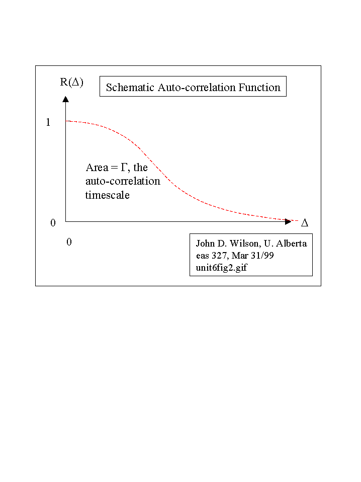
Consider a section of a fluctuating signal y(t). We will assume the signal y(t) is "stationary," meaning that its average properties (such as its variance σy2) are not drifting in time. For such a signal we can define the autocovariance as the average value of the product of the signal at one time (t) with its value at a different time (t + Δ). The autocorrelation is that number made dimensionless by dividing by the variance σy2. Thus the autocorrelation R(Δ ) is defined to be:
R (Δ) = ⟨ y(t) y ( t + Δ) ⟩ / σy2
where the angle brackets denote the average value of the quantity they enclose. As implied by the notation R(Δ ), R is independent of the reference point t, and depends only on the time "lag" Δ.
The schematic autocorrelation function shows that, necessarily, R(0)=1, ie. that R(Δ) = 1 when Δ =0. It is also intuitively clear that R(Δ) ---> 0 at very large time-separations Δ . To give a physical example, if the wind is blowing up now, in all probability it will still be blowing up 1 microsecond from now - but we have no idea whether up or down one hour from now.
Now Δ has units of time. So the area under the graph is a time. This area is called "the autocorrelation timescale" (Γ), and is a good estimator of the time over which the signal y(t) becomes decorrelated from itself. If we take samples at intervals exceeding Γ, those samples will be independent.
8.0 Sampling Distribution of the Mean: the Central Limit Theorem
If random variable x belongs to (any) probability distribution having mean μ and variance σ2 then, according to the "Central Limit Theorem" an average
⟨x⟩ = 1/N Σi xi
has a "sampling distribution" which is "asymptotically" Gaussian with mean μ and variance σ2/N.
What does this mean? Well the mean value ⟨x⟩ is itself random, since the xi are random. In different trials we will get different sample means < x >. So < x > itself has a probability distribution. Provided N is "large" (say > 15; thus the proviso "asymptotically") that distribution is Gaussian (=Normal) with mean μ and variance σ2/N.
9.0 Confidence in Measurements of a Random Variable
Suppose I want to estimate the true average value of a fluctuating variable x(t) over an interval spanning t=(0,T). My estimate is a sample mean, mx = < x > (these are just alternative notations for a sample mean). How many measurements (N) must I take to ensure that with 95% probability (ie. in 95% of all such experiments) my sample mean
⟨x⟩ = 1/N Σi xm(i Δt)
lies in the range μ ± ε? Here xm(i Δt) = xmi is the measured value of x (which may differ from x, for example if our instrument is too slow to respond to rapid fluctuations in the signal x) at time t=i Δt, where Δt is the "sampling interval" or "time between samples." And ε is the error band.
The notation xm emphasizes that our measured x's are not necessarily equal to the true x's. We can assume our instrument is accurate, in the sense that if it is presented for a very long period of time with a steady value of x then it measures xm=x. In the jargon, the device has correct "DC" or steady state response. But we will assume it is not infinitely fast - it is characterised by a time constant τ, so that if presented with a step change in x it will achieve only 66% response in time τ, and 95% response in 3τ. Therefore, we must distinguish xmi (the measurement at time i) from the true value x(ti). In particular, this means that our measured sample standard deviation (smx) may well be different from the true standard deviation σx. If our instrument is "slow" then smx < σx, while if our instrument is very noisy, perhaps smx > σx.
The CLT (Central Limit Theorem) tells us that if I was to perform this exercise many times, ie. determine mx many times, then my population of measured means would cluster in a Gaussian distribution, centred on the true (population) mean μ, and with standard deviation smx/N½.
Now we know that a Gaussian distribution (the "bell-shaped curve") has 66% of its area within ±1 standard deviation from the mean, 95% within ±2 standard deviations, 99% within ±3 standard deviations. It follows that provided the number of samples N determining the mean ⟨x⟩ is "large," with 95% probability ⟨x⟩ lies in the range μ ± 2 smx/ N½
We can rearrange this result to give the answer to our starting question ... if I take
N >= 4 (smx/ε)2 measurements, then with 95% probability (ie. in 95% of all such experiments) my sample mean ⟨x⟩ = 1/N Σi xm(i Δt) lies in the range μ ± ε.The slower our instrument, the smaller will be our measured variance smx2 and thus the smaller is the required number of samples.
The only restriction on this result is that the samples xi must be independent. How do we ensure they are? What if we packed a million measurements of x into a microsecond? Intuition says they would not be independent. But can we be quantitative about it? Yes. By appealing to the concept of the autocorrelation (self-correlation) of a signal x(t) and the corresponding autocorrelation timescale: if the samples are separated in time by intervals Δt greatly exceeding the autocorrelation timescale, they are independent.
Back to the Earth & Atmospheric Sciences home page.