Objective will be to have you able to:
1.0 Introduction
An anemometer measures wind velocity (a vector) or speed. In these notes I will distinguish a vector by using bold font; thus, the velocity vector is u and, if referred to the usual rectangular Cartesian axes has three components which are typically named:
u = ( u,v,w)
The three velocity components are the projections of the velocity vector along directions (x,y,z), where the meteorological convention for naming axes & velocities is to choose z vertical (w the vertical velocity component) and x parallel to the average wind (u the alongwind component). We will call the magnitude of the wind vector V,
V = { u2 + v2 + w2 }½
and we will call the speed in the horizontal plane (the "cup" windspeed, so called because in principle that is what is "seen" or measured by a cup anemometer) s,
s = { u2 + v2}½
2.0 Anemometer Specifications:
The following is not an exhaustive list:
A sensor can only provide us information on the flow in which it is imbedded if it interacts with the flow. In the categories below are mentioned several anemometers which we will explore later in detail.
This figure shows a pitot tube connected to a manometer. You may have seen these on aircraft. Note that there is no flow in the tubes because they are blocked by the pressure transducer, whether it be a simple manometer or an electronic sensor based (eg.) on deflection of a membrane acting as one plate of a capacitor. If there is no flow in a tube, the pressure is constant along it - so the tubes simply carry a pressure "signal" to each side of a pressure transducer.
A key point is that the pitot tube measures velocity correctly only when the velocity vector is parallel (or very close to parallel) to its shaft. In that condition the velocity near the front port is zero - and that point is called a "stagnation point." The approaching air is deflected away from that point, by an adverse pressure gradient. The pressure at that front tip, the "stagnation pressure" ps, exceeds the background "static" pressure po by an amount
ps - po = ½ ρ u2
where ρ is the air (or more generally the flowing fluid) density and u is the speed. In using this formula, you must use consistent units, preferably MKS. Please note that this formula, which gives us a very general and useful result that is unaffected by details of the geometry of the pitot tube, can be derived from the priciples of fluid mechanics. More-refined formulae exist, that take account of specific geometry of the probe, the Reynolds number of the flow, and such details.
The pressure at the "static port(s)" is po, because the wind there is not impinging on the tube, but flowing parallel. So the pitot tube creates and transfers to a pressure transducer the pressure difference ps-po. Thus if we can measure ps-po we can deduce u. The pitot tube is therefore absolute (although the pressure transducer may need to be calibrated unless it is absolute itself, eg. a manometer). It is also non-linear. Remember that the density ρ is easy to calculate from the pressure p [Pa] and temperature T [oK].
Numerical example: if u=1 m/s, and remembering ρ is about 1 kg/m3, we get ps-po=½ [Pa]. Atmospheric pressure is of order 105 Pa. This is a minute pressure difference. Can we measure it?
Let's consider our transducer to be a manometer, whose tube has cross-sectional area A and whose fluid is water, density ρw=1000 [kg m-3]. The higher pressure ps on one side displaces upwards a small column of water of height h. Now at a constant level in the water the pressure is constant. Thus we know that column of height h is held up by (ie. its weight, A h ρw g, is balanced by) a force which is simply (ps-po)A, the pressure difference acting on area A.
A (ps-po) = A (ps-po) = A h ρw g
A cancels. We see that h measures (ps-po). That is the principle of a manometer.
So how big is h for our ½ Pa pressure rise when u=1 m/s?
h = (ps-po)/(ρw g) = ½/(1000 10) = 5x10⁻⁵ m = .05 mm.
Immeasurable. But if u=10 m/s, we increase this result by 102/12 = 100. The result, h=5mm, is an easily measureable displacement of the water column. Thus we see that the pitot will be a marginal device at very low speeds, but a good tool at medium speeds. In practise one usually uses an electronic pressure transducer, probably calibrated against a manometer. One can purchase at moderate cost very sensitive differential transducers, having a full scale pressure differential as small as 0.1 "H2O (that pressure excess causing h=0.1" for a water manometer). Note that a pressure of 1" H2O is equivalent 249.2 Pa.
Summary: The pitot-tube is non-linear, absolute, suitable only for uni-directional flow at moderate speeds. Variations such as the "pressure sphere" anemometer overcome the angular limitation.
5.0 The cup anemometer
The cup anemometer is not a high fidelity instrument. It does not measure s, or even the average value of s, exactly. Many articles have analysed errors of cup anemometers. Nevertheless, due to their quite low cost (though one pays around US$700 for a very good cup anemometer) they remain the usual choice for many types of wind measurements near ground.
The analysis below follows Wyngaard (1981; Ann. Rev. Fluid Mech. 13, p399). The linked figure shows an anemometer having cups of frontal diameter d whose centres rotate on a circle of radius r. The cups have angular velocity dθ/dt and linear velocity uc=r dθ/dt , while the true windspeed in the horizontal plane is s. Typical cup anemometers have r/d in the range (1 -> 1.25) and uc/s in the range (0.3 -> 0.5).
The governing principle of the cup anemometer is that angular momentum is conserved. In words, "moment of inertia (I) times angular acceleration (d2θ/dt2 ) equals net torque acting (τ)."
What is moment of inertia? For a device like this having axial symmetry it is the sum of the masses of the cups times the square of their distance from the axis of rotation (we are neglecting the contribution of the shafts supporting the cups, but it could easily be calculated):
I = S m r2 ~ 10-4 kg m2.
So the governing equation is:
I d2θ/dt2 = τd - τf
where τd is the torque due to the drag of the wind on the device and τf is the friction torque (bearing friction, generator torque if a generator is attached to the shaft, etc).
Steady state analysis: If the wind is steady (and therefore the angular acceleration of the cup is zero) and we neglect friction, the governing equation reduces to τd=0 (thus the inertia is irrelevant; this is always the case in the context of steady-state response).
Now we will adopt a "model" for τd based on the two-cup simplification ( 2-cup model). The cups have cross-sectional area A. The front side of a cup has drag coefficient cdf while the back has cdb, with cdf>cdb. That cup facing into the wind and moving sympathetically downwind is pushed by a force
ρ A cdf (s-uc)2
while the other, driven back against the wind so that the relative velocity is s+uc, is pushed by a force
ρ A cdb (s+uc)2
Then the drag torque, force times distance from the axis of rotation, is
τd= 0 = r ρ A [ cdf ( s - uc)2 - cdb ( s + uc )2]
A couple of lines of algebra will now show that the steady state calibration factor g=uc/s is governed by:
g2 - 2 G g + 1 = 0
where
G = (cdf + cdb)/(cdf-cdb) = (1+e)/(1-e)
where e=cdb/cdf < 1. This is a quadratic equation for the steady state calibration factor g=uc/s (remember that the anemometer output is proportional to uc, whether it be a number of pulses per revolution, perhaps 1, or a DC voltage proportional to rotation rate). The remarkable thing is that the calibration does not depend on the air density. Who would have guessed? The cup anemometer responds to wind forces, and those wind forces have a magnitude directly proportional to density. Yet because in a steady state those forces are balanced, density vanishes as a factor.
If e=¾, g=14±195½, while if e=½, g=3±8½. In both theses cases we have two real positive solutions for g=uc/s, one large and one very small. These are ostensibly eligible solutions; but for any e, it would have been more satisfying to find only one real root. Never mind, our model is an oversimplification.
We won't go on to look at the dynamic response (response to sudden changes). But it can be shown that a cup anemometer in turbulent flow overestimates the mean speed ("overspeeds") because it accelerates more rapidly in gusts than it decelerates in lulls (example of cup overspeeding error; observations from an open flat field at Ellerslie, Alberta, May 2003; Wilson, in press, J. Applied Meteorol). Cups also have a "w-error," a departure from true cosine response (Hyson 1972; J App. Met. 11, p843), perhaps as large as a 6% error at heights of around 4 m. Other analyses of cup anemometers and their various errors are given by:
6.0 The Wind Vane and the 'Potentiometer'
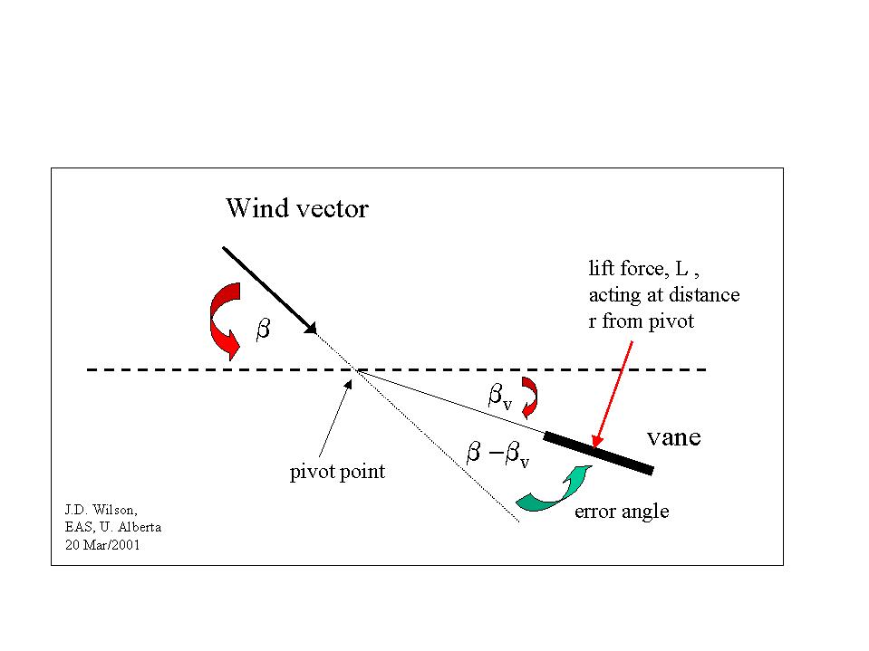
We shall consider the response of a wind vane to a (small) step change in wind direction. The equation of motion is again the statement that angular momentum is conserved, ie.
I d2βv/dt2 = L r
where d2βv/dt2 is the second derivative in time of the vane angle (the rate of change of the rate of change of the vane angle, ie. the angular acceleration), and L is the component of the lift force on the vane acting perpendicular to the vane at distance r from the pivot.
Now assume the lift force (L, [N]), which is non-zero from the instant the step change in direction occurs, can be written:
L = A CL ρ V2
where A is the area of the vane, ρ is air density, V is the magnitude of the wind velocity (ie. the speed), and CL is a dimensionless lift coefficient.
We further assume the lift coefficient varies linearly with the 'error-angle' of the vane, ie. difference between vane angle βv and wind angle β,
CL = α ( β - βv) .
Now our equation of motion can be written
d2βv/dt2 = ( β - βv) / τ2
where the time scale
τ = ( I / α ρ r A V2)1/2
has not the same interpretation as it does for a first-order system. Note that if windspeed V=0, the rate of response is zero... this makes sense.
We now want to solve this 2nd-order ordinary differential equation, with the (2) initial conditions that:
and we enforce (t > 0), β = const. = B
Using the standard method for linear ode's with constant coefficients, it is straightforward to show that:
βv = B [ 1 - cos (t/τ)]
ie. the vane oscillates about the desired angle B with amplitude B. The addition of a damping force into the analysis (a term in the governing equation proportional to - dβv /dt alters this result, so that the oscillation is "damped.").
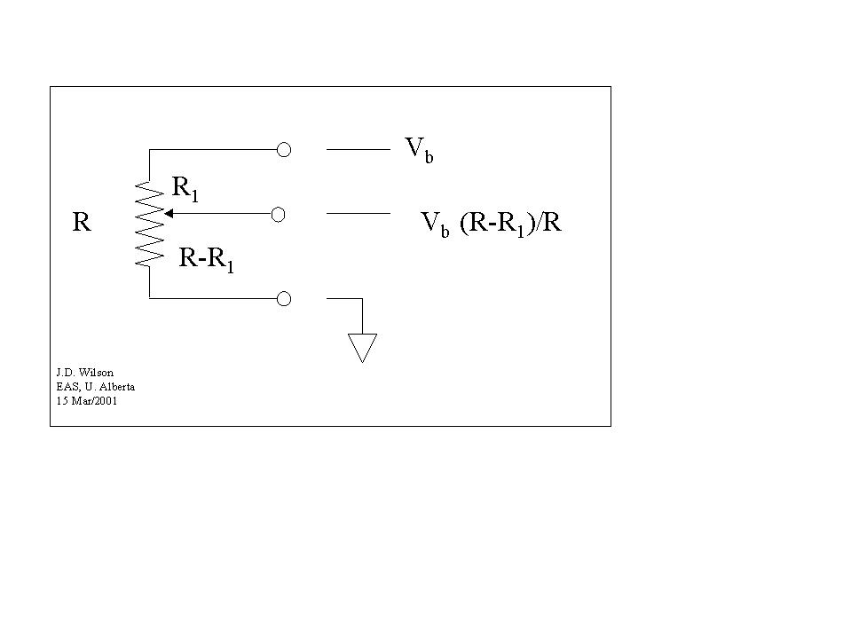
The electronic signal output from a wind vane derives, usually, from a "rotary potentiometer." A potentiometer is a three-terminal resistor, in which one of the terminals is a "tapping point," or "wiper", dividing the total resistance (R) into two parts (shown as R1 and R-R1). A rotary pot is simply a potentiometer connected to a shaft, such that when the shaft turns the wiper moves from top to bottom of the resistor, ie. R1 varies from 0 to R. Accordingly, the signal from the rotary pot varies from 0 to Vb.
Inevitably there is a "dead band" of angles within which the wiper makes no connection with the resistor (typically the dead band may be about 10o wide). One sets up a wind vane so that, for wind directions of interest, the wiper does not lie within the dead band.
7.0 The Propellor anemometer
The propellor anemometer has a relatively low cost, is simple and reliable to operate, and so has proven popular both for measuring the mean flow and the turbulence. Typically the prop drives a DC generator, and so the output is a millivolt-level DC voltage, proportional to windspeed. In principle the prop measures the axial wind component, though in practise the cosine response is imperfect (errors are discussed below).
For turbulence measurements, three propellors are often set in an orthogonal array. For more routine windspeed measurements, the "prop-vane" is a popular choice - a single propellor mounted on a vane. In this latter case the propellor rotation rate gives the instantaneous magnitude (s) of the horizontal component of the wind vector
s = { u2 + v2}½
while a rotary potentiometer (variable resistor) attached to the shaft of the wind vane gives wind direction
β = tan-1 (v/u)
with respect to the x axis.
Dynamical model of a Propellor Anemometer
A feature of the propellor anemometer that has been noted by EAS students when calibrating propellor and cup anemometers side-by-side in the wind tunnel, is the much faster rotation rate of the propellor. Can we explain this?
In order to understand the factors determining the rate of rotation of a propellor in a steady wind, we shall invoke a simplified Model of the Propellor Anemometer, namely, a flat plate in wind-driven linear motion along a single axis (y). The figure shows this plate (propellor blade), mounted and free to move on a track parallel to the y-axis. This y-track runs perpendicular to the wind U, which is directed along the x-axis. In response to a steady wind vector (U) that is oriented perpendular to the track (ie. pointing along x), the blade will move, at a velocity we shall denote v, along the track towards increasing y. We let U denote the magnitude of U (ie., bold denotes a vector).
The angle θ struck by the plate relative to the y-axis is a design parameter, and corresponds to the pitch of the propellor blade (though a propellor blade, like an aircraft prop, has a pitch that varies with radius, for reasons we explore below). We shall suppose the pitch angle θ to be non-zero (else there would be no preferred direction of slide); designing θ small and positive will ensure v > 0 (motion to the right). Then, if the plate was prevented from moving along y, the angle of attack α of the wind (its deviation from being parallel to the plate) would take the value α = (π/2 - θ) .
But a propellor anemometer does rotate, and so for our model to be reasonable, we must permit the blade to slide along the y-axis in response to any force in that direction. But, due to the resulting motion of the plate itself along y, the relative velocity between the plate and the air is not given by the vector U. As you can see from the vector-addition triangle, the magnitude of the relative velocity is (U2 + v2)½, while the direction of the relative wind is tilted away from the x axis, through angle φ, which is given by:
φ = arctan (v/U)
Consequently, the relative wind vector is closer to being parallel to the plate, than it would be if the plate were stationary: ie. the angle of attack α of the wind on the plate is reduced due to the plate velocity v, and is given by:
α = (π/2 - θ) - φ
Now, let FD and FL be the components of the aerodynamic (wind) force on the plate along the x and y directions, and let Ff be the bearing friction. We need have no interest in FD, as it is perpendicular to the motion. Now, if we assume stationarity (ie. steady wind and steady motion), the net force acting must vanish:
FL + Ff = 0.
We can model the track (bearing) friction as Ff = μ v. The aerodynamic lifting force FL can be modelled as:
FL = CL(α) A ρ (U2 + v2)
where A is the area of the plate, ρ is the air density, and CL = CL(α) is the dimensionless coefficient of lift. For a flat plate, the lift coefficient CL vanishes when the angle of attack α = 0. Therefore provided α is small, we can approximate CL as:
CL = CL0 sin α ∼ CL0 α .
So our force balance is:
CL0α A ρ (U2 + v2) - μ v = 0
and upon dividing through by CL0Aρ and substituting for α we have
[(π/2 - θ) - arctan (v/U) ] (U2 + v2) - μ (CL0 A ρ)-1 v = 0
Suppose now we neglect bearing friction. Then μ = 0, and our solution (the calibration) is:
v/U = tan ( π/2 - θ).
The calibration equation indicates the steady state plate velocity is that which ensures that angle of attack vanishes and lift force disappears. This is the key to understanding the propellor anemometer. It is interesting (and very significant for the practicality of the anemometer) that, just as for the cup anemometer, the steady-state calibration factor is independent of air density ρ. We needn't account for any p,T dependence of our calibration factor (which is useful to know: for in Canada, with an annual temperature range that may exceed -40o <= T <= + 35o, fractional variation in ρ is not insignificant).
In fact we can do slightly better than to totally neglect bearing friction. Suppose instead we retain friction, and simply note that according to observations, v >> U. Dividing our dynamical equation by v2 we have
[(π/2 - θ) - arctan (v/U) ] (1 + U2/v2) - μ (CL0 A ρ v)-1 = 0
Now letting v be large, we recover the same calibration, v/U = tan(π/2-θ).
Suppose the design pitch angle θ=10o (if we held the plate from moving, the angle of attack would be 10o). Substituting into our calibration equation,
(v/U)(θ=10) = tan (90o - 10o) = 5.67 ,
while for a shallower design pitch angle θ=5o, (v/U)= 11.4. We have confirmed that the propellor anemometer does indeed spin faster than a cup anemometer.
How does this relate to a real prop-anemometer? There is no fundamental reason not to build a prop anemometer using a single prop... but the resulting net drag torque (due to the aerodynamic drag force FD acting at a single point off the axis of rotation) on the bearing would be inelegant and presumably demand a more expensive bearing than needed - so why not use multiple propellors, thus balancing the drag-torque,ie. for a two-bladed propellor τD = r.FD-r.FD=0. The only other feature of real propellor anemometers that needs comment, is the fact that, just as with aircraft propellors, one notes a variable pitch of the blade. In effect, the design pitch angle θ gets smaller at greater radial distance r from the axis of rotation. This is easily understood as being due to the fact that, since the propellor spins as a solid body at angular velocity ω, the propellor "runaway velocity" (v, in our plate model) increases linearly with radius r, ie. v = r ω. Thus, for a fixed wind speed U and propellor rotation rate ω, the deviation (φ) in angle of attack increases with radius,
φ = φ(r) = arctan(ω/U r)
Then, in order to have the lift force vanish at every point along the radius of the blade at a specified (fixed) ω/U, one needs to vary the pitch angle θ along the radius, ie. construct θ = θ(r) so that:
α = 0 = (π/2 - θ) - arctan(ω/U r).
So the propellor blade must have its pitch vary with radius r to ensure that:
θ = π/2 - arctan[(ω/U) r].
Propellor Anemometer Errors
There are three types of errors: cosine response error, threshold error, and inertia error. Threshold and inertia place a severe limitation on use of a prop to measure w - the propellor anemometer is suitable only at large heights (say 50 m or more). All three types of errors are thoroughly discussed by Horst (1973; J. Appl. Meteorol. 12, p716), who gave an iterative algorithm for correcting the errors due to deviation from cosine response - but which can only be used if all three velocity components are being measured.
Can any of these errors be reduced or eliminated?
Inertia error limits the frequency response of the prop anemometer, ie. due to its inertia the prop fails to record the fastest fluctuations of windspeed. Of course the inertial error (directly related to the moment of inertia I, as defined above for the cup anemometer) is determined entirely by the mass distribution of the propellor with respect to its axis, and is not amenable to reduction other than by reducing the size and weight or the blades.
Threshold error can be eliminated by providing "air bearings," which ensure that there is no friction when the prop is not turning, and only the viscous friction of a layer of air while the prop spins (negligible).
Another means to reduce or eliminate threshold error is to tilt the propellor array off-horizontal and into the wind, so that no propellor need be changing its direction of rotation, ie. crossing its threshold speed. This is rather inelegant and a nuisance, since wind direction β is highly variable and unpredictable - in what direction does one tilt the array? Both threshold error and cosine error are practically eliminated in the case of the prop-vane. However inertia (both of prop and vane) continues to compromise measurement of faster fluctuations by a prop-vane.
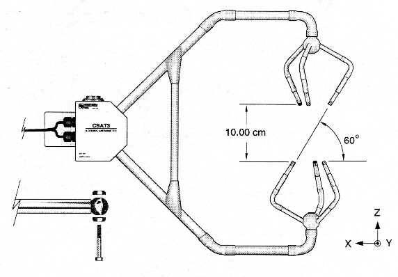
8.0 Sonic Anemometer
The sonic anemometer exploits the fact that a train of sound waves (usually ultra-sound) travels in a fluid at a velocity (relative to fixed axes) that is the SUM of the intrinsic speed (c) of propogation of sound in still fluid, PLUS the bulk convective velocity of the fluid with respect to the axes.
The speed of sound in a gas (pressure p, density ρ) is
c = (g p/ρ)1/2
where g=cp/cv (ratio of specific heats at constant pressure and constant volume). Taking g=1.405 (the value for N2), we have c [m/s] = 20.081 T1/2, but here I have been a little sloppy or inconsistent in that I used the dry gas constant for air (287)... If I was more careful, the result would be:
c [m/s] = 20.067 T1/2
where T is air temperature [Kelvin] and a small dependence on humidity and total pressure has been neglected.
Now imagine a pulse (P1) of sound travelling vertically downward over distance d (the pathlength) from a speaker (these days, often a piezoelectric transducer that functions efficiently either as a highly tuned source, or as an efficient receiver of tuned ultrasound), and a reverse pulse (P2) taking the opposite path. If we define the vertical wind velocity w to be positive for upward motion, than the travel times will be:
P1 (down): t1 = d / (c-w)
P2 (up): t2 = d / (c+w)
Then
1/t2 - 1/t1 = (2/d) w
while
1/t2 + 1/t1 = (2/d) c
So the sonic gives us both velocity (along the path) and temperature (ultrasonic anemometer-thermometer). The device is instantaneous, ie. has no inertia since there are no moving parts (any inertia is due to the speed of the electronics), and linear.
By providing two paths in the horizontal plane (2d-sonic) one may obtain the two horizontal components u,v, or equivalently s = { u2 + v2}½ and the wind direction β=tan-1(v/u). A 3-d sonic provides all three velocity components.
9.0 The Hot Wire/Film
The hot film/wire anemometer dates back to early this century. In the "constant temperature" version, a very fine wire (or a cylindrical metal film on a glass rod or tube) is controlled at about 250 oK above ambient temperature. The convective heat loss to the airstream is balanced by Joule heating. Thus the electrical heat supply is a measure of the airstream velocity (with a correctable influence due to the temperature difference).
The operating Reynolds number of these devices is typically about 10. This is very small because the wire is so fine (order 5 μm). Of course such a fine wire has minute heat capacity, so that the hot wire has phenomenal frequency response - out to perhaps 1000 Hz or more. This is essential for wind tunnel turbulence measurements, superfluous for atmospheric measurements. However the hot wire is only used in a research mode in the atmosphere, as it is delicate, requires calibration frequently, and needs a skilled and attentive operator.
Assume the resistance of the actual hot wire, which is held suspended in a fork, varies linearly as
R=Ro(1+ α(T-To)) where Ro, To, and α will be specified by the supplier of the sensor. We settle on a desired value Top for the operating temperature (say 250 oC) and this formula implies a corresponding operating resistance Rop. We want to control R as closely as possible to R=Rop. How?
The hot wire is placed in a Wheatstone bridge, as in the Figure. The error amplifier (receiver of the bridge imbalance signal) produces an output voltage Vo=A(V+-V-) where A is an enormous number. This output is then returned (a feedback) as the bridge voltage. Applying our knowledge of voltage dividers:
V- = R/(R+R2) Vo , V+=Rc/(Rc + R1) Vo
Therefore:
Vo = A Vo [ Rc/(Rc + R1) - R/(R+R2) ]
Dividing out by Vo we conclude that since A is infinite the factor in brackets on the RHS is zero. The bridge is held in balance; therefore (easily shown) R=RcR2/R1. The feedback holds the bridge in balance, so if R1, R2, and Rc are chosen right, R can be controlled at R=Rop - and therefore the sensor is held at exactly the desired (very high) temperature.
How do we get our velocity information? Let P [Joules/s=Watts] be the rate of provision of electrical power to the hot wire. Since the hot wire temperature is steady, its energy balance is of the form:
P = Area ( QH + Q*)
where QH is the convective heat flux density and Q* the radiative. We neglect the latter, and model the convective heat flux density as:
QH = h(u) (Top-Ta)
Here h(u) is the (windspeed-dependent) heat transfer coefficient (we could have introduced a Nusselt number), which under usual operating conditions (Re order 10, etc) can be approximated as
h(u)= a + b u½
where a and b are constants to be determined by calibration. Ta is the air temperature. Note that small fluctuations in Ta of order a few degrees imply fluctuations in Top-Ta of say (3/230)x100 = 1%.
Now the power P is simply:
P = (V-)2/Rop = Vo2 G
where G =Rop/(Rop+R2)2 is just a constant. Then
Vo2 G / (Top - Ta) = h(u) = a + b u½
We see that the square of our signal voltage Vo is proportional to the square root of the windspeed. The hot wire is very non-linear.
Problems? There is an angular sensitivity. The above analysis is fine if the wind lies in the plane normal to the wire, but there is not a cosine response as the wind is turned to have an along wire component. Clearly if the wind is perfectly aligned with the wire there is still heat loss, so still an apparent velocity. To resolve wind direction, 3 such wires are needed. That is a considerable complication. Also, there is a threshold. With such a big wire-air temperature difference, at very low windspeeds (say below about 30 cm/s) buoyancy forces come into play, a factor not considered in our analysis. Despite these problems, in very complex turbulent flows such as within vegetation, the multiple-element hot wire/film anemometer has been the only possible choice until the recent advent of a short path-length (10 cm) 3-dimensional sonic anemometer.
Back to the Earth & Atmospheric Sciences home page.