2.0 Introduction
All the sensors we use (temperature, humidity, windspeed) must somehow be "coupled" to the environment (else they would be unable to provide us with information on that environment, whether it be air, water or soil). The coupling is most commonly by way of exchange of mass or energy. The following theory of that exchange is fairly general; however there are some built-in superficialities, eg., a "bulk" treatment (eg. a given "object" is treated as having a single surface temperature).
We are talking about "transport" of heat, mass, etc. in physical systems. Do you recall Fourier's law of heat conduction? Fick's law of molecular diffusion? If not, please review the appendix on the conduction and diffusion laws of Fourier and Fick.
These laws do not describe the world at the microscopic level (the level of the motion of individual atoms or molecules), but rather are empirical macroscopic laws, that describe the observable outcome of the unseen microscopic process. The form of these laws is:
Flow ("flux") .proportional to . spatial gradient (or difference) in "driving force"
eg. the existence of a temperature difference within a (conductive) medium causes heat to flow; the existence of a pressure difference along an open tube causes fluid to flow; and, the existence of a voltage difference across a (finite, ie. conducting) resistor causes charge to flow.
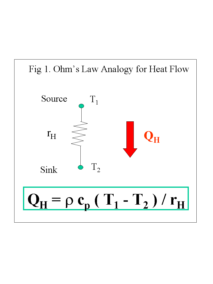
2.1 The Ohm's Law Analogy
We will treat energy and mass exchange between a fluid and an immersed object by what is known as "the Ohm's Law analogy." All other treatments of the problem are equivalent, though mathematically they may differ superficially (eg. one can choose to use conductivity instead of resistance; but the two are reciprocal).
We postulate a source (the object), and a sink (the fluid surrounding the object). Between the two, there is some "resistance" to flow of the property in question.
Consider specifically the Ohm's Law Analogy for Heat Transport. We measure the rate of flow of heat away from the surface of the source by a "sensible heat flux density," and give it the symbol QH [J m-2 s-1 = W m-2]. QH measures the number of Joules [J] of (heat) energy lost (gained) by the source, and therefore gained (lost) by the sink, per unit of surface area of the body, per unit of time. The Ohm's Law analogy is:
QH = ρ cp (T1-T2)/rH
Here ρ [kg m-3] is the density of the fluid; assuming the fluid is air, then given the pressure and temperature, we are able to calculate ρ from the ideal gas law. And cp is the specific heat (at constant pressure) of the fluid: we may obtain this from tables. The key variable in the equation is rH [s m-1], which is called the "transfer resistance."
Now note that not very much has been accomplished. We have transferred our ignorance of the heat exchange rate (for given temperature difference) to an ignorance of the numerical value of the coefficient rH. In effect, all we have done is to write down an equation that defines a new unknown, rH. However it is an equation whose form is sensible. There is reason to hope that sensible rules might therefore exist for the specification of rH. By the way, rH has units of [1/velocity]. People often work with a conductivity gH=1/rH instead.
Note that we have committed ourselves here to a "bulk treatment." Only two temperatures have been admitted, T1 and T2, whereas in any real physical system, there is a continuous distribution of temperature. Of course, more sophistocated analyses are possible... but this (the bulk treatment) is sufficient to our purposes.
Now, the Ohm's Law analogy for Mass Flow. We measure the rate of flow of mass away from the surface of the source by a "mass flux density," and give it the symbol Qm [kg m-2 s-1]. Qm measures the number of kilograms of mass lost (gained) by the source, and therefore gained (lost) by the sink, per unit of surface area of the body, per unit of time. The Ohm's Law analogy is:
Qm = (C1 - C2)/rm
where C is the mass concentration [kg m-3], and rm is the transfer resistance (again, units s m-1) for the particular species of mass being exchanged. Though it will suffice for our purposes in this course, this law for mass transfer is not always valid: a more careful specification of the driving force (here simply the concentration C) is sometimes required.
The mass flow of most concern to us, is water vapour exchange (eg., wet bulb temperature sensor). Then, C is the what we call the "absolute humidity," or the "vapour density," ρv (for information on the common variables for measurement of vapour content in the environment, follow Water Vapour Variables). We will give the water vapour flux density the special symbol E (evaporative flux density), and we have:
E = (ρv1 - ρv2)/rV
Latent Heat Flow. If I give you one kilogram of water vapour, you can extract from that about 2.5 x 10⁶ Joules of energy, simply by condensing the vapour, and trapping the latent heat released. Thus a flux density of water vapour implies a flux density of energy, called the latent heat flux density, and given the symbol QE. For every a [kg] of water vapour transferred, L a [J] of energy are transferred, where L [J kg-1]= (about) 2.5 x 10⁶ is the latent heat of vapourisation (L is a weak function of temperature; and if the source or sink is frozen, we need instead the latent heat of sublimation). Using the ideal gas laws for the air in total (p= ρ R T) and for the water vapour (e = ρv Rv T) you can easily show that:
QE = LE = (ρ cp/ γ) (e1-e2)/rV
where γ = p cp / ( 0.622 L ) is called the "psychrometric constant," but misleadingly so, because it is not constant! Clearly it depends on p; and also, weakly, on temperature, through L. The factor 0.622 is the ratio e = R/Rv of the specific gas constant for air (about R = 287 J kg-1 K-1) to the specific gas constant for water vapour (Rv = 462 J kg-1 K-1).
We have already covered the ground work to accomplish an analysis of, eg., the wet-bulb thermometer. But first, we will take this further.
2.2 DIMENSIONLESS FORMULATION of Heat (and mass) Transfer
In any equation that describes the physical world, all terms must have the same dimensions. If I write A + B - C = D, then necessarily [A] = [B] = [C] = [D]. The equation must be "dimensionally homogeneous." If S is a "scale" for quantities having the dimensions of A (etc.), I could rewrite the equation in dimensionless form:
A/S + B/S - C/S = D/S
Often by recasting physical laws in dimensionless form, we can achieve a very useful simplification.
The example of interest to us is heat transfer to/from a body in a moving fluid stream. The Nusselt number is defined to be "the ratio of the actual heat flux density to that which would occur if the same temperature difference (T1-T2) was imposed on a still fluid layer of depth d, where d is a "characteristic dimension" of the body."
Numerically, the Nusselt number is:
Nu =QH / { ρ cp DH (T1 - T2)/d }
where DH [m2 s-1] is the thermal diffusivity of the fluid, easily found from tables.
For bodies of simple enough geometry (spheres, discs, flat plates,...) it is a very useful empirical fact that Nu = Nu (Re, Gr), where Re and Gr are another pair of dimensionless numbers, the "Reynolds number" and the Grashof number. The Reynolds number is an indicator of the ratio of inertial to viscous forces in the flow,
Re = U d / ν
where U is the fluid velocity about the body, and ν [m2 s-1] is the "kinematic viscosity" of the fluid (available from tables). The Grashof number indicates the importance of buoyancy forces in the flow, and is given by:
Gr = { g d3 (T1 - T2 ) }/ { 273 ν2}
Convective heat exchange between a body and a fluid is classified as being: fully forced convection, mixed convection, free convection. In fully forced convection, buoyancy forces due to the temperature difference betwen the body and the bulk airstream exert no influence on the flow around the body; in free convection, buoyancy forces control the flow aboput the body, and any the background (bulk) fluid velocity is irrelevant; between these extremes we have mixed convection, in which case the flow about the body is affected both by the overall motion of the airstream about the body (background flow) and by buoynacy forces which locally perturb the motion. Criteria for categorizing the type of convection are:
Forced Convection: Gr < 0.1 Re2, then Nu=Nu(Re)
Mixed Convection: 0.1 Re2 < Gr < 16 Re2, then Nu= Nu (Re, Gr)
Free Convection: Gr > 16 Re2, then Nu= Nu(Gr)
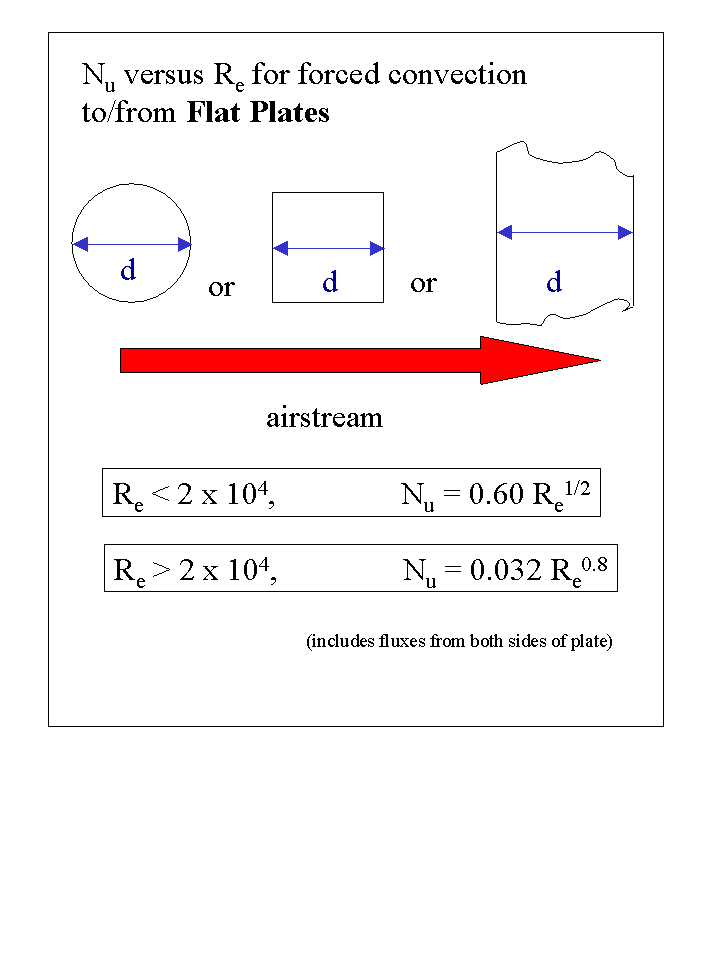
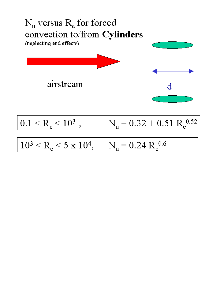
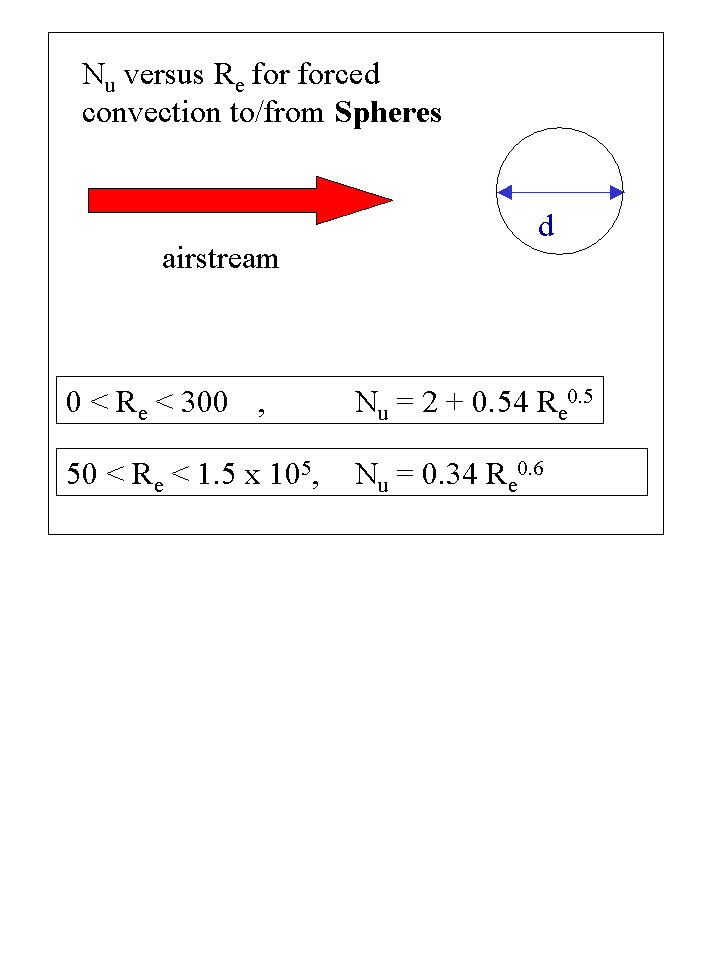
Follow these links for empirical Nu vs. Re correlations for heat transfer in forced convection from
For such bodies, this information in effect gives us the coefficient rH we introduced earlier as the key unknown. To see this, note that we can write the equation for the heat flux in the following equivalent forms:
QH = ρ cp (T1-T2)/rH = h (T1-T2) = ρ cp DH Nu (T1-T2) / d
where h is the "heat transfer coefficient." What it boils down to is, once we know Nu we can evaluate QH by means of
rH = d/(DH Nu)
or
h = cp DH Nu/d
Back to the Earth & Atmospheric Sciences home page.