EAS372 -- Lecture Log -- 2015

• Thurs 9 April. Downscaling a reanalysis: the July 1996 Big Freeze in Southern New Zealand

• Tues 7 April. Weather briefing (Dana and Scott). Exercises:
  1. assess each other's weekend forecasts, relative to the observations: provide constructive feedback by firstly identifying/confirming the evidence (that was available at the time) that you consider supports each aspect of the original forecast, and any forecast element that appears to lack apparent basis; and secondly, indicate which aspects of the forecast were confirmed by observations and which (if any) were not.
  2. using correct grammar, sum up the weather situation as of 12Z in C. Alberta in one brief paragraph.
  3. in the above (given) data, what evidence suggests there are two distinct air layers over C. Alberta having differing (recent) histories? Is there any evidence to justify a suggestion that the sky condition indicated by the Tory web camera might be representative of a broad area over C. Alberta? -- and is there any evidence to the contrary?
  4. relating to the above "two histories" conjecture, and time permitting, compute 48h back trajectories ending at 12Z this morning at 500 m and at (say) 2 km AGL).
  5. complete last week's exercise, "calibrate the constant α in the TKE eqn..." [Solution has been added to file as of 16 April.]

  Added after class: 48h back trajectories ending at YEG 06Z Tues 7 April at 3000 m AGL and at 500 m AGL.

• Thurs 2 April. NCEP's NWP models.

  Exercises:

  1. determine the LCL and the LNB for the Prince George sounding (00Z 2 April 2015; hard copy distributed), regarding which this morning's MSC forecasters' discussion makes mention [Marked up sounding, added 17 April.]
  2. prepare a forecast (NWP allowed) for conditions along the Edmonton-Calgary corridor, valid from Saturday morning through Sunday evening. Might there be any issues for drivers? [Files added to verification_data.html collect guidance available at the time, and document conditions observed.]

• Tues 31 Mar. Weather briefing (Sean and Tyler). Finish file on "NWP: CMC's GDPS, RDPS & HRDPS".

  Exercises:

  1. use spotwx.com/ to create a table conveniently comparing forecasts by HRDPS West, RAP and NAM for wind direction, wind speed, surface temperature and fractional cloud cover at 18MDT today for Lacombe, Alberta (see table added after class, at verification_data.html)
  2. calibrate the constant "α" in the TKE eqn. (see file)

• Thurs 26 Mar. Weather briefing (Samantha and Tory). Continue "NWP: CMC's GDPS, RDPS & HRDPS."

  Exercises:

  1. Hand in a paragraph summarizing the 12Z meteorological situation as it pertains to central Alberta's weather this morning.

     Instructor's diagnosis as of 9MDT: moist upper flow rounding a ridge axis centred over central BC, resulting in moderate humid NW wind aloft over C. Ab. Overcast (SCu). Weak surface trough in Ab. resembling lee trough; slack isobaric gradient, arctic high much further east, centred in Manitoba. Mild surface temps and light easterly (or calm) surface winds. [Some relevant charts.]

  2. Evaluate the vertical gradient in mean potential temperature, supposing that (at a certain height z) the unresolved kinematic vertical heat flux density was 0.2 [m s^-1 K] and the eddy diffusivity was K_h=5 [m² s^-1].

• Tues 24 Mar. NWP: CMC's GDPS, RDPS & HRDPS.

  Exercises:

  1. assess forecasts of last Thurs. versus data for valid time (18Z Sat. 21 March). Write a paragraph that summarizes the weather at valid time, in qualitative terms.

     Instructor's summary: firm (circa 20 kph, or stronger) surface easterly (upslope) out of artic ridge (ridge axis running NW-SE through Saskatchewan). Overcast (SCu). Not very cold (minus 5). Recent snow. Southerly aloft, and humid, but no strong vertical motion. Sounding quite stable, surface easterly beneath upper humid southerly.

  2. catch up on exercises of last week

• Thurs 19 Mar. Satellite meteorology.

  Exercises:

  1. Prepare a forecast for C. Alberta valid at 18Z Saturday 21 March (use of NWP permitted). [Archive of progs available for the forecast].
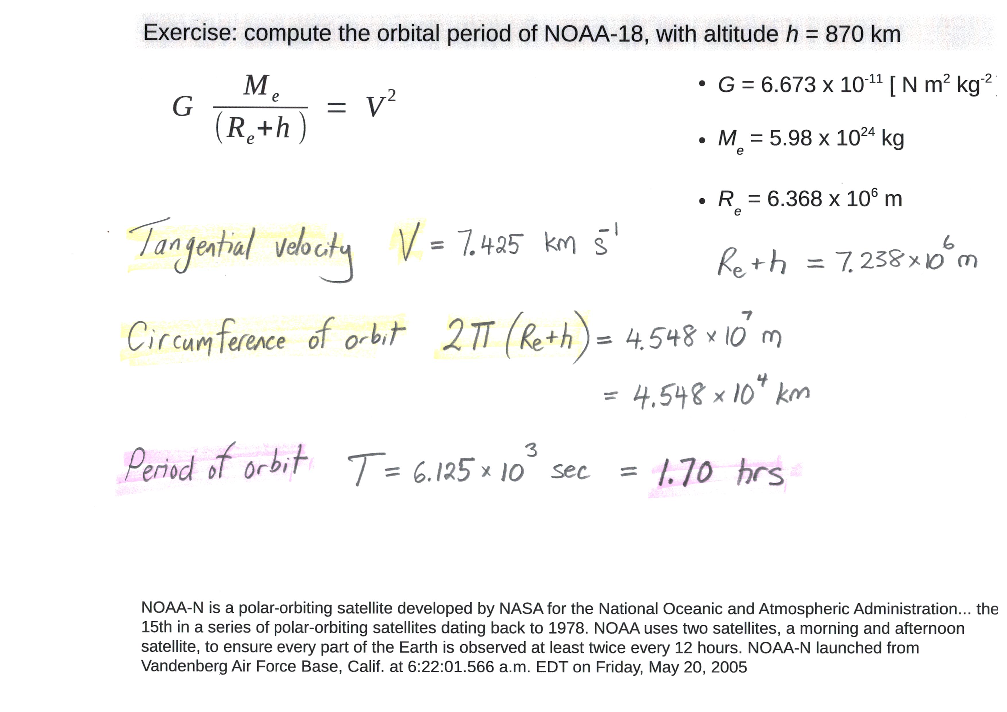
  2. Orbit calculation (see Satellite meteo. file)

     Answer: orbit calculation.

• Tues 17 Mar. The ideal (horizontally homogeneous; unsaturated) atmospheric surface layer (continued).

  Exercises: ABL heat budget; and surface layer wind profile. (Handout: 2 cycle log-linear graph paper; the higher cycle on the log axis is truncated before completing. 3-cycle semi-log graph paper.)

  Answers:

  • Heat budget questions (angle bracket denotes average): (1) surface kinematic heat flux ⟨w'θ'⟩₀ ≈ 0.28 K m s^-1; (2) ∂⟨θ⟩ / ∂t ≈ 0.6 K hr^-1
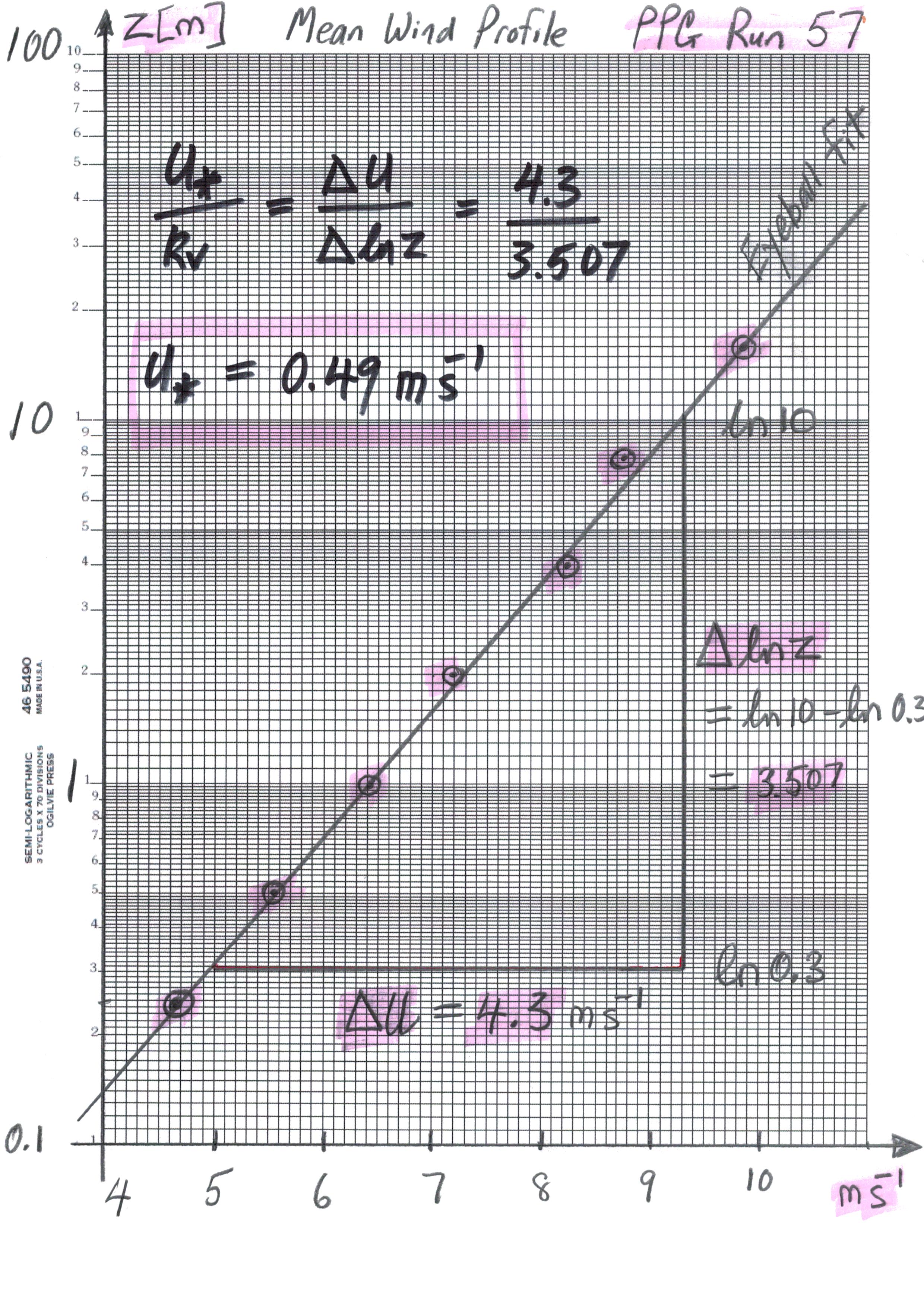
  • Graph of mean wind profile for PPG Run 57, and computation of friction velocity
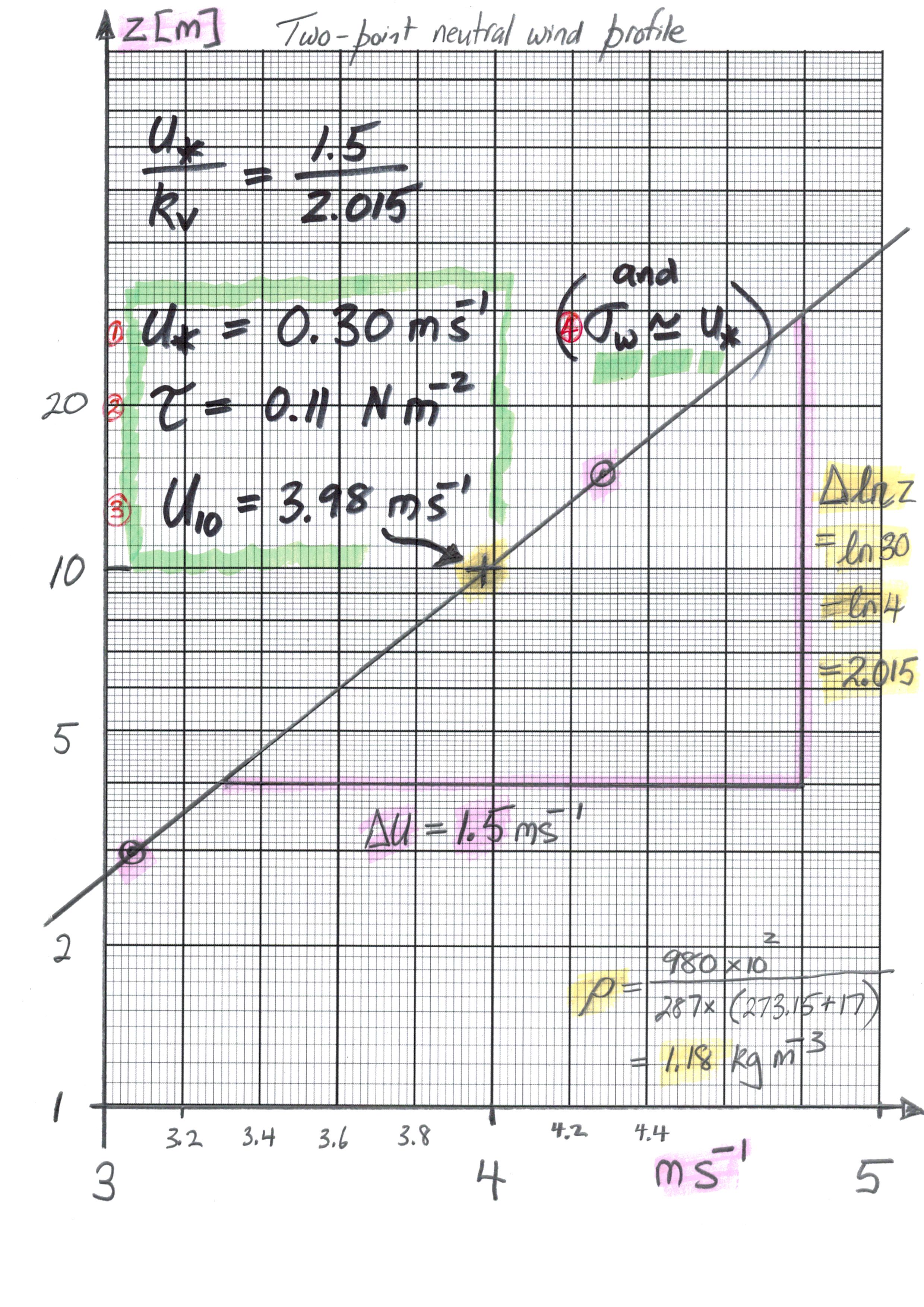
  • Graph of two point mean wind profile, and computation of friction velocity, surface drag, 10 m wind speed and standard deviation (σ_w) of vertical velocity
  • Note on extracting Δln(z): observe that ln(10)-ln(1) = 2.30259 = ln(8)-ln(0.8) = ... Thus one decade on the paper always has the same ruler length (say, "D"), and this ruler distance corresponds to the constant ln(10). Thus, measure the length D on your graph paper and the length d correspondingto your interval on the ln(z) axis. Then Δln(z)=2.30259 (d/D). [It is usually quicker to use your calculator to obtain the difference ln(z₂)-ln(z₁)].

• Thurs 12 Mar.: Parameterizing effects of transport by unresolved scales of motion (continued from Tuesday 10 Mar). Introduction to the ideal atmospheric surface layer (context for Assignment 3).

  Exercise: Estimate the rate of advection of absolute vorticity at the points indicated.

  Sample: Instructor's result. You'll have noticed that there is much discretion available in which pair of contours you choose, what is the orientation of the s-n unit vectors, and so on: thus the sizeable estimates of uncertainty indicated.

• Tues 10 Mar.:
  1. The Q-vector formulation of the QG omega equation (modified after class)
  2. A look ahead at a fast-moving storm (possibly of interest as subject for Assignment 3)
  3. Model "physics" versus model "dynamics" in NWP: treatment of the influence of unresolved scales of motion. Explicit separation of resolved and unresolved scales of motion by way of the Reynolds average. Eddy fluxes. Reynolds-averaged heat equation and momentum equation.

• Thurs 5 Mar. The ageostrophic wind, isallobars and the isallobaric wind.

  Exercises:

  1. Briefly evaluate your own 24h forecast against observations for 12Z yesterday (Wed. 4 March), data given below

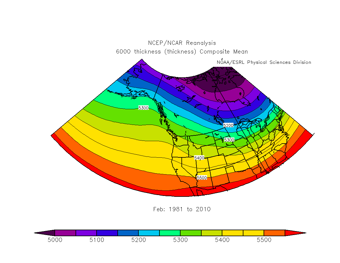
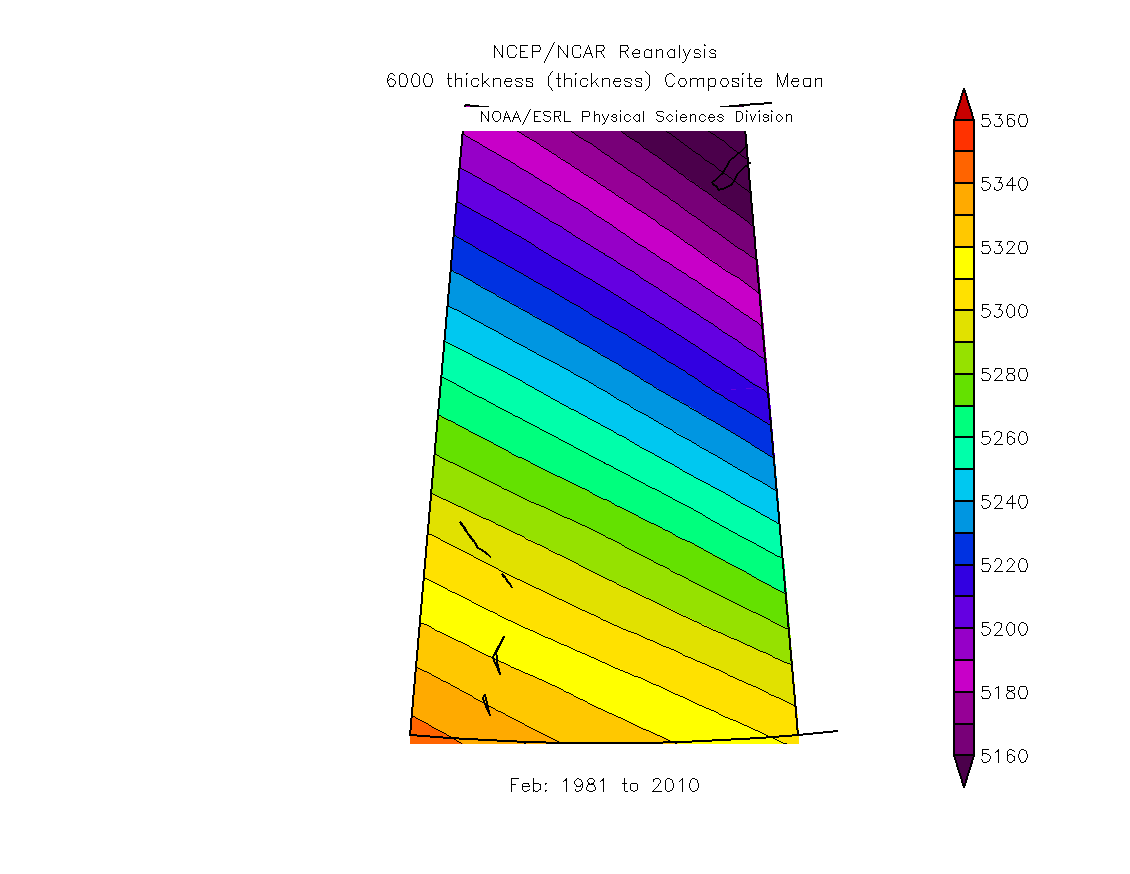
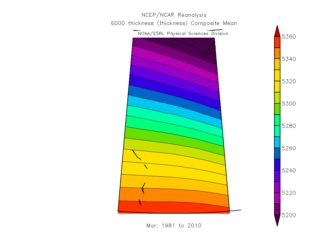
  2. Determine the spatial pattern of the climatological (30-yr mean) 1000-500 hPa thickness over Western Canada for February, by creating a chart by the procedure below (time permitting, repeat for March). Compare the climatological mean thickness over Alberta with the observed thickness as of Tuesday.

     Procedure:

     • www.esrl.noaa.gov/psd/cgi-bin/data/getpage.pl
     • Type of analysis: Climatology
     • Time Scale: monthly
     • Time range: any
     • Variable: Other
     • Dataset: NCEP/NCAR Reanalysis
     • Show web pages
     • Select: "Monthly/Seasonal Maps and Composites: NCEP/NCAR Reanalysis and other datasets
       • Which variable: Thickness
       • Level: Thickness (1000 to 500 mb)
       • Beginning and Ending Month: Feb
       • Enter range of years: 1981 to 2010
       • Plot type: mean
       • Scale plot size: 200%
       • Map projection: Custom
       • Lowest lat: 30
       • Highest lat: 70
       • Western-most longitude: 190
       • Eastern-most longitude: 290
       • To zoom in on Alberta, choose latitude range 49 to 60, longitude range 240 to 250
     • Create Plot

     Examples:

     • February, wider area
     • February, Alberta focus
     • March, Alberta focus
     The normal thickness for February over C. Alberta is about 526-527 dam, but at 12Z on Thurs 5 March the thickness over C. Alberta was between 504 and 510 dam, i.e. at least 16 dam "colder" than normal. For March, the normal thickness is about 529 dam (interpolating to the right spot on these figures is a bit tricky).

• Tues 3 Mar. Velocity deformation, fronts and frontogenesis; and examples.

  Exercise:

  • Based on this morning's 12Z analyses (but no progs!), prepare your own forecast for C. Alberta valid 12Z Wed. 4 March. Mark up this cropped CMC 500 hPa analysis (valid 12Z today) in whatever manner best guides your thinking. Here are some very broad ideas as to a possible procedure.

  • Instructor's examples (24h fcst, no NWP):
    • Forecast valid 12Z Wed 4 March ["Clear. Light NW sfc wind. Low -15 to -22. Thickness increase by 6-12 dam"]. Based (strictly) on CMC analyses for 12Z Tuesday ("t₀") at the surface, 850 hPa, 700 hPa and 500 hPa, along with the 500 hPa analysis from 24 h earlier (t₀-24).

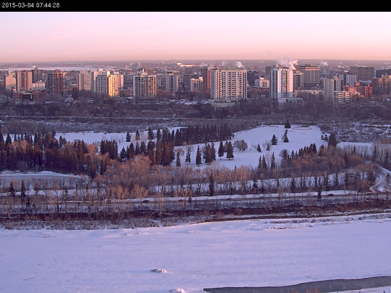
      Verification data: Edmonton 07 MST (and past 24 h); Tory webcam at 0740 MST; CYEG 041200Z 18010KT 15SM SKC M21/M26 A3013 RMK SLP266= ; CMC surface, 850 hPa, 700 hPa and 500 hPa analyses for 12Z Tues 4 March. Forecast assessment: Surface wind observed to be southerly rather than NW (consistent with the sfc isobar pattern, and at 10 knots one might say "firm" rather than "light". Otherwise the forecast was qualitatively correct: thickness did increase (from about 508 to 522 dam, i.e. by ~ 14 dam); YEG reported -21^oC and clear at 12Z.

      "PRAIRIE AND ARCTIC STORM PREDICTION CENTRE OF ENVIRONMENT CANADA AT 7:00 AM CST WEDNESDAY MARCH 4 2015... UPPER RIDGE FROM BRITISH COLUMBIA UP THROUGH THE MACKENZIE BASIN. AN IMPULSE IS DEPRESSING THE TOP OF THE UPPER RIDGE AS IT APPROACHES BANKS ISLAND. THIS IMPULSE IS SUPPORTING A SURFACE LOW OVER THE BEAUFORT SEA WITH A TROUGH ALL THE WAY SOUTHWARDS ACROSS WESTERN ALBERTA. EAST OF THE LOW, AN ELONGATED SURFACE RIDGE EXTENDS FROM THE CENTRAL ARCTIC SOUTH THROUGH WESTERN SASKATCHEWAN AND INTO MONTANA, WITH PLENTY OF COLD AIR ASSOCIATED."

    • Forecast valid 12Z Tues 3 March ["For YED 12Z Tues. Light sfc wind. Cooler thickness by 2 cntrs (12 dam). Clear sky. Low -20 or milder"]. This was based (strictly) on CMC analyses for 12Z Monday ("t₀") at the surface, 700 hPa and 500 hPa, along with the 500 hPa analysis from 24 h earlier (t₀-24).

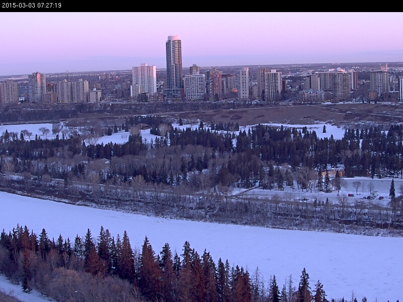
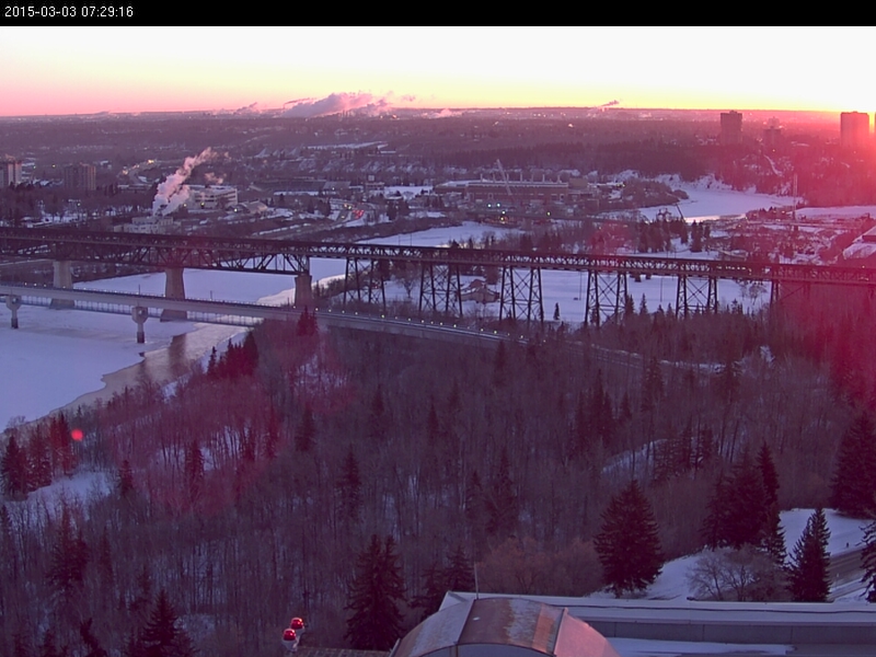
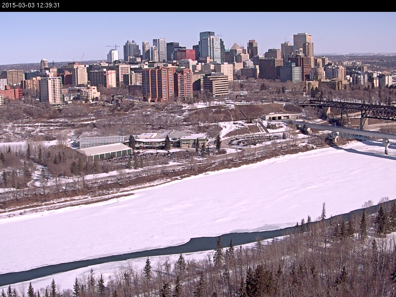
      Verification data: observed conditions at Edmonton International Airport "METAR CYEG 031200Z 29008KT 15SM SKC M19/M24 A3023 RMK SLP300=", public weather statement Edmonton 06 MST, Tory webcam images 0730 MST looking north and east. CMC surface and 500 hPa analyses for 12Z Tues 3 March. Forecast assessment: qualitatively correct. The 500 hPa stream did move eastward, cold advection easing off (due to realignment of thickness and height contours to reflect thermal wind balance); the arctic high (surface system) did expand over AB; skies were clear, we did have a fairly frigid overnight low (helped by longwave radiative cooling); the surface wind was light (as of 12Z), though liable to pick up (webcam images show the industrial plumes bending); thickness fell, by something like 8 dam. A fine day ensued (Tory webcam 12:30 MST looking northeast.)

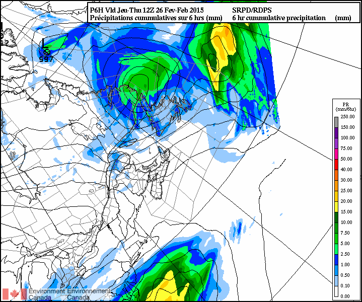
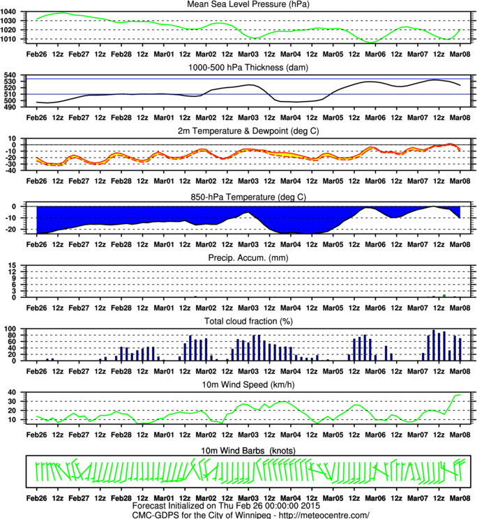
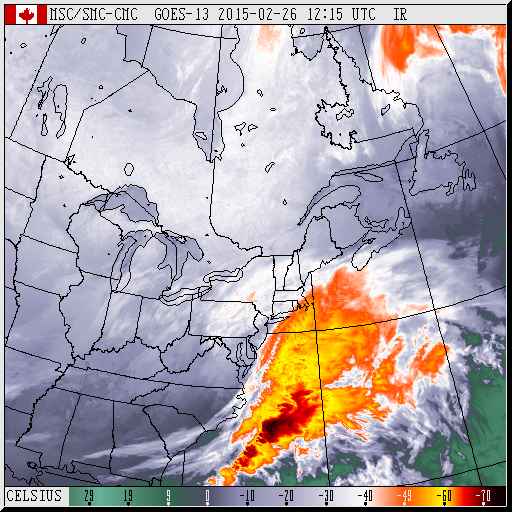
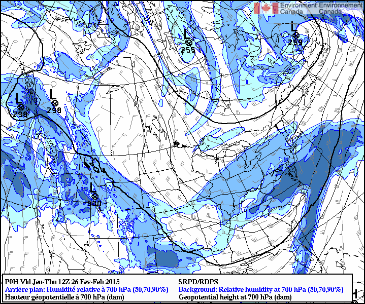
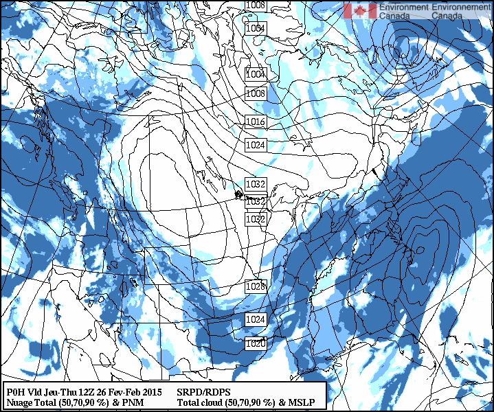
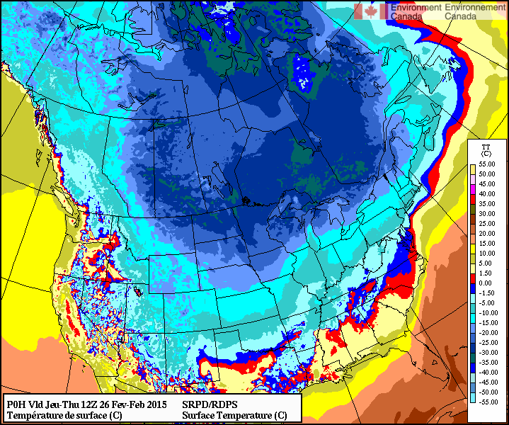
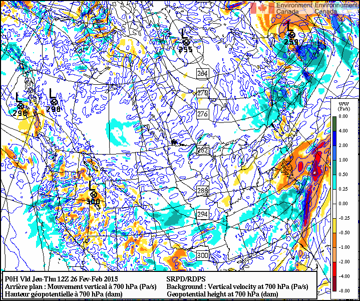
• Thurs 26 Feb. Midterm exam (with answers).

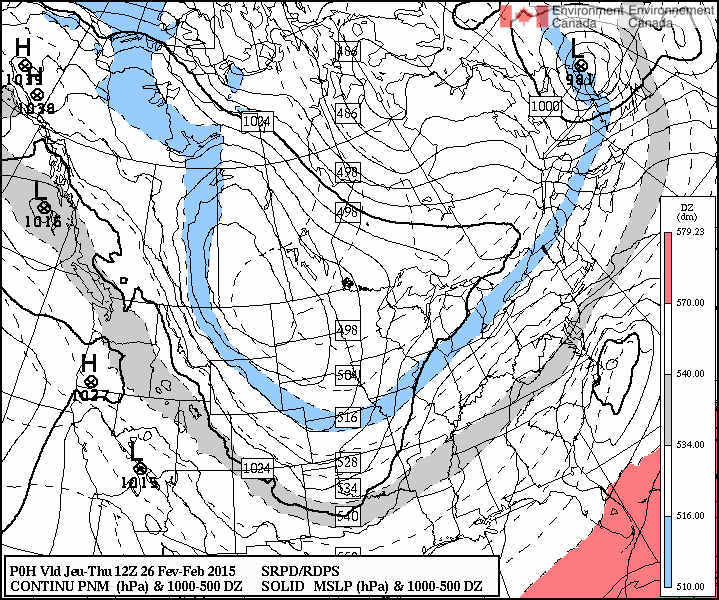
  The following maps/data are relevant to the "Live web weather data" component of the exam:

  • RDPS 0h prog valid 12Z: MSLP & thickness
  • RDPS 6h prog valid 12Z: 6h cumulative precip (Domain: East Coast)
  • NAM 6h prog valid 12Z: 6h cumulative precip
  • GDPS prog initialized 00Z: meteogram for Winnipeg
  • GOES East 1215Z: IR image
  • METAR for CYYC at 12Z: CYYC 261200Z 17010KT 5SM -SN BKN008 OVC035 M14/M16 A3032 RMK SC6SC2 SLP352=
  • Sounding for YQD (The Pas) at 12Z: Data

  The following maps/data are relevant to the "Interpretation of Weather Charts" component of the exam:

  • RDPS 0h prog valid 12Z: 700 hPa height & RH
  • RDPS 0h prog valid 12Z: Total cloud
  • RDPS 0h prog valid 12Z: MSLP & thickness
  • RDPS 0h prog valid 12Z: Surface temperature
  • RDPS 0h prog valid 12Z: Omega at 700 hPa
  • RDPS 12h prog valid 12Z: 12h cumulative precip

• Error estimation: Suppose the "absolute" uncertainty (or error) in A is the quantity a, and in B it is b. Here a has the same units as A and b has the same units as B. We then say that the "relative" error (or "fractional error") in A is a/A, and, obviously, the "percentage error" in A is 100a/A.

  Now, we'd like to be able to state the error in combinations like A+B or A-B or AB or A/B. This is done as follows:

  • the absolute error in a sum or difference, A+B or A-B, is the sum of the absolute errors, a+b. Thus

    (A ± a) + (B ± b) = (A+B) ± (a+b), and,

    (A ± a) - (B ± b) = (A-B) ± (a+b).

  • however to get the error in A*B or A/B we must add the "relative errors" to get the fractional error in the product or quotient. The relative error in A*B or A/B or B/A is (a/A+ b/B). And if we want the absolute error in A*B or A/B we simply multiply the result by the fractional error. So, for example

    (A ± a) × (B ± b) = AB × [1 ± (a/A + b/B)].

    You can equally well combine percentage errors instead of "relative" errors... a percentage error of 10% is a relative error of 0.1.

    So if the percentage error in A is 10% and in B is 25%, the percentage error in A*B or B/A or A/B is 35%.

  Now suppose A=2 with a=0.4 (percentage uncertainty 20%) and B=1.5 with b=.5 (percentage uncertainty 33%). Then

  A - B = 0.5 ± 0.9.

• Tues. 24 Feb. The meteorology associated with a fatal wind storm in central Alberta (sudden extreme wind gusts of 19 Dec. 2004).

  Exercises:

  1. Using NOAA's HYSPLIT application, create an ensemble of 48 h backward trajectories, ending at CYQD (The Pas, Manitoba) at 06Z today. Compare with 48 h trajectories ending CYEG at 06Z yesterday. Qualitatively, do the trajectories to some extent explain weather conditions at The Pas and at CYEG?

     Examples: trajectories to CYQD (The Pas) at 06Z Thurs. 26 Feb. 2015, and trajectories to CYEG (Edmonton Int'l Airport) at 06Z Mon. 23 Feb. 2015. (Note: these are based on forecast wind fields from a prog that was initialized at 0Z Feb. 22.)

  2. Assess your forecast (prepared in class Thurs. 11 Feb.) against observed conditions 00Z Wednesday 18 Feb. 2015. Some of the maps that were available on Thurs. 11 Feb. when you made your forecast, as well as a set of charts depicting the actual conditions at or around the target time (or "valid time") for your forecasts, are collected in verification_data.html.

• Thurs. 11 Feb. Continuing the quasi-geostrophic model (file updated 5 Mar.): the QG height tendency equation.

  Exercises:

  1. Please hand in your brief forecast of weather conditions for a location of interest to you, valid nominally at 00Z Wednesday 18 Feb. Include a broad estimate of surface temperature range; describe the most significant aspects of the upper flow (700 hPa) and the lower tropospheric (850 hPa) thermal pattern; identify any significant surface pressure system and front(s); likelihood of precipitation in a time window of many hours (say, nominally, plus or minus six hours) from 00Z Wednesday 18 Feb.

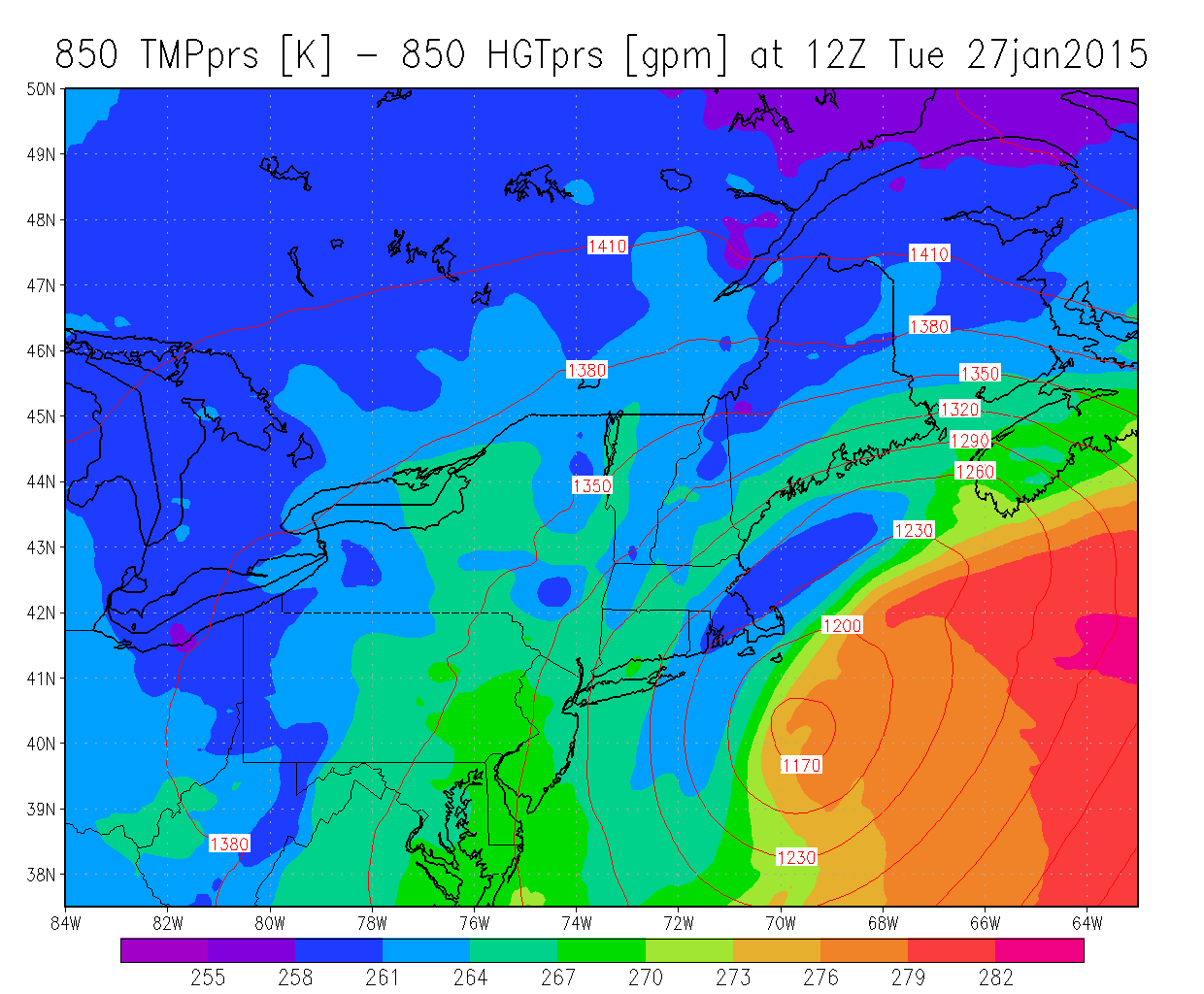
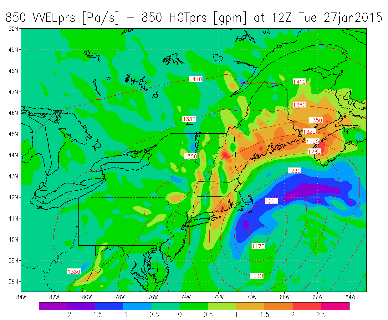
  2. Revisiting the New York snow storm of 27 Jan. 2015, please regenerate NAM 0h progs valid at 12Z that day from the archive at http://nomads.ncdc.noaa.gov/ (needed steps given below). Choose those maps you'd consider most useful in order for a meteorologist to get a quick idea of the meteorological situation, e.g. isobaric height, temperature and vertical velocity at the 850 hPa and 700 hPa levels. Other maps may be of interest (e.g. precipitable water).
     • go to http://nomads.ncdc.noaa.gov/
     • Access → NAM → Near real time & historical NAM, Plot | FTP4u → Select date range, Cycle (1200), Forecast Hours (0000), select Generate Quick Plots, Submit data request → Plot data → Advanced users, select dataset (upper option), select "Overlay two variables" → next page → Select your two "parameters" (fields)... it seems to work best to make your height field the second variable, eg. to get 850 hPa height & temperature contours
       • Parameter 1 settings: "air temperature, pressure levels [K] - 39 levels", vertical level 850 millibars
       • Parameter 2 settings: "geopotential height -[gpm] - 39 levels", vertical level 850 millibars
       • Optionally adjust countour intervals and line types/colours to suit your taste
       • Map Region: NE USA
     • Here's an example of a regenerated 850 hPa analysis and the corresponding omega field. Note that the 850 hPa height contours have been plotted at a 3 dam interval rather than the usual 6 dam of CMC charts. Can you assess whether vertical motion was frontal or convective?
     • On the basis of your charts, can you explain why New York City received only a modest snowfall amount (roughly 10-20 cm), amounting to much less than had been feared? (Note that if one had the time and the interest one might retrospectively regenerate the sequence of NAM analyses (always 0h), and track the evolution of the storm as it ran up the coast.)

• Tues. 10 Feb. The quasi-geostrophic model (file updated 5 Mar.), and an example of its use.

  Exercises:

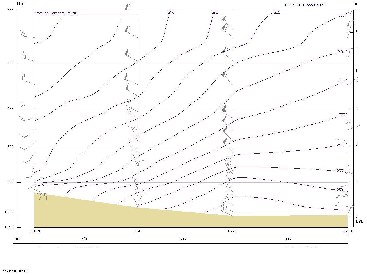
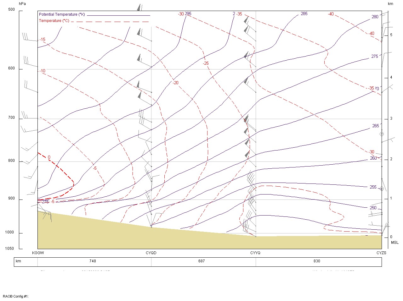
  1. plot isotherms for T=(-40,-35,-30,-25,-20,-15,-10,-5,0)^oC in order to complete this (T, θ) vs. p cross-section (hard-copy handout, isentropes already plotted) for 12Z Monday 9 Feb. 2015, a transect running (approximately) NNE from Glasgow (Montana) through The Pas and Churchill (Manitoba) to Coral Harbour, i.e. GGW/YQD/YYQ/YZS. Procedure: from the radiosonde data at these stations
     • ggw_20150209@12Z_data.pdf
     • yqd_20150209@12Z_data.pdf
     • yyq_20150209@12Z_data.pdf
     • yzs_20150209@12Z_data.pdf

     determine at what value of p each isotherm crosses the station; then interpolate smoothly between stations. Note that some isotherms will intersect the ground. The CMC 850 hPa analysis for 12Z Monday 9 Feb. 2015 indicates a transect at along the 850 hPa level will cross something like seven isotherms.

     Completed cross-section (plotted by Windows package "RAOB"). Itersection of isotherms and isentropes results in quadrilaterals that are termed "solendoids." The rate of temperature advection is inversely proportional to the area of the solenoids (smaller quadrilaterals, stronger thermal advection).

  2. determine the static stability σ = - (R_d T / p) ∂lnθ/∂p at 700 hPa over The Pas (YQD)

     Results: The RAOB cross-section suggests looking for the heights of the "isentropes" for θ=290 K and θ=285 K. From the sounding data at The Pas (YQD), 289.6 K occurs at 681 hPa and 286 K at 719 hPa. Taking these figures, ∂lnθ/∂p ≈ [ln(289.6)-ln(286)]/[(681-719)x100]= - 0.0125/3800 [Pa^-1]. Since T₇₀₀=259 K, we have σ = (287 x 259 / 70000) x 0.0125/3800 = 3.5 x 10^-6 [Pa^-2 m² s^-2]. Holton (2004, Chapter 5, p150) gives σ=2.5 x 10^-6 [Pa^-2 m² s^-2] as a mid-tropospheric value for the standard atmosphere.

• Thurs. 5 Feb. Comment on Assignment 1. Weather briefing. Action of the Laplacian operator (preliminary for covering the Quasi-Qeostrophic model).

  Exercises:

  1. Today's 12Z surface analysis indicates upslope flow in C. Alberta, e.g the surface wind is a NE at 5 m s^-1 at Edmonton (please confirm this against a CYEG Metar). Given the elevations of Edmonton (nominally 670 m ASL) and Rocky Mountain House (990 m ASL), and the straightline distance between them (about 160 km, with Rocky M.H. roughly SW of Edmonton) deduce: (i) the mean slope as an angle and as a percentage, (ii) the ascent rate w [m hr^-1] of a surface parcel moving from Edmonton towards Rocky at 5 m s^-1, and (iii) the implied cooling rate of that parcel (to keep things simple, assume the parcel is not saturated)

     Answer: (i) mean slope is α=0.115^o, or 0.20%. (ii) the ascent rate is w=5 sin α ≈ .01 m s^-1. (iii) in one hour, a parcel travelling along its surface path climbs a distance of about d= .01 x 3600 = 36 m. The implied cooling rate is 36/100 K hr^-1, or in view of the approximate nature of the calculation, let's say 1/2 K hr^-1. One can see why upslope motion is significant in terms of producing a saturated layer, possibly resulting in fog or even precip.

  2. As prep for the QG model, a little challenge. Let y be a local coordinate pointing northward, at latitude φ=φ₀. Find an expression for the derivative (df/dy)_φ0, in terms φ₀, earth's rotation rate Ω and earth's radius R

     Answer: Use the chain rule df/dy=df/dφ x dφ/dy, noting that dy=R dφ.

• Tues. 3 Feb. Review Skew-T diagram (families of curves, etc). Relating the thermal wind to the sounding and the hodograph, with examples (courtesy of UCAR) for 12Z today from Glasgow, Montana and Bismarck, N. Dakota: compare the orientation of the implied thermal wind with isotherms near these stations on the 850 hPa analysis. Work required (or liberated) in displacing a parcel along the vertical. CAPE and CIN, and their identification on the Skew-T chart.

  Exercises:

  1. Plot a hodograph for Sable Island (WSA) for 10 Jan 2015 at 12Z (latitude 44^oN, off the east coast; JDW has added a ring around this station on the 850 hPa analysis). At a minimum, plot the radiosonde winds at 1000, 850, 806, 747 and 700 hPa (maybe use pencil, if this is unfamiliar). Plot a thermal wind vector V_T for the 850 to 700 hPa layer. Relative to Sable Island, what compass direction would you take to find colder air? Compare the orientation of your V_T vector with the isotherms at 850 hPa and the thickness contours (0h bw prog). Are your findings consistent with the thermal wind equation (Eqs 1.42, 1.43)? Note: the "heel" of the wind vector for each and every level you plot is (implicitly) at the origin, and you plot a point for the "head of the wind vector. The thermal wind vector connects any pair of points, and is directed towards the higher of the two.

     Result: WSA sounding (and data); the corresponding hodograph with thermal wind vector for 850/700 hPa layer.

  2. Acknowledging that time was scarce, that you may have consulted charts/guidance differing from those collected below, and that the forecast objective given you was very broad, let's anyway take time to reassess our forecast from last Thursday --- against the following evidence:
     • The surface analyses for 06Z and 12Z: northerly winds out of the arctic high, snowing.
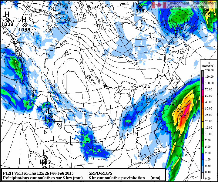
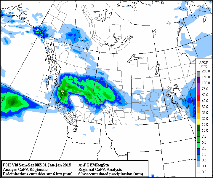
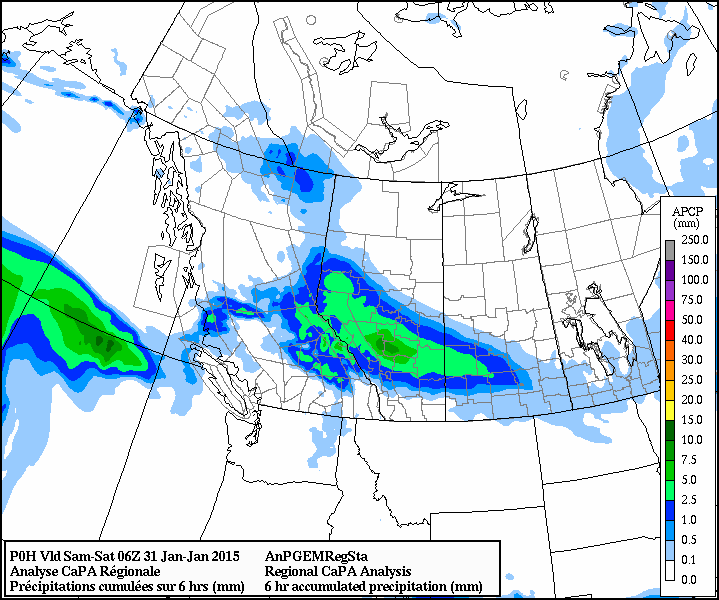
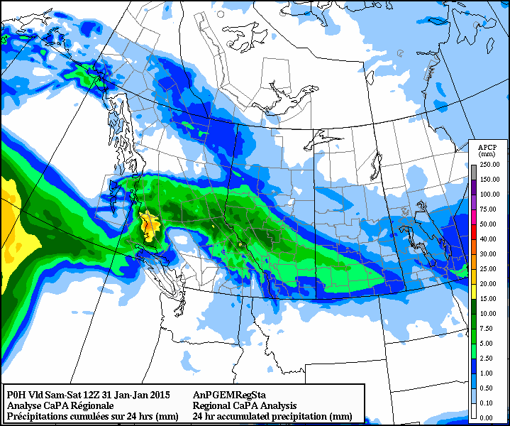
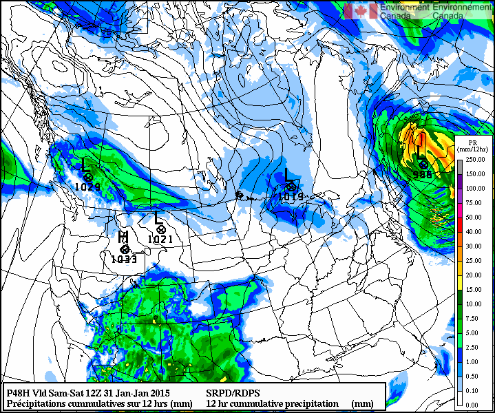
     • The CaPa precipitation analyses: 6hr cumulative precip as of 00Z Saturday and as of 06Z Saturday; and the 24hr cumulative precip as of 12Z Saturday... below 10 mm (liquid equiv.) for our area, which, taking the usual multiplier implies about 10 cm of snow (for snow falling in cold conditions a larger multiplier of 15 is sometimes taken).
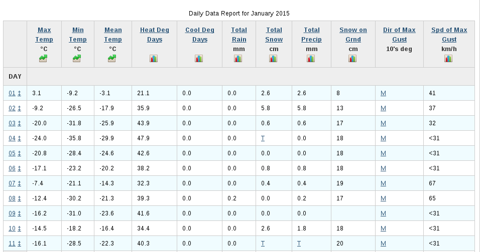
     • This is consistent with the recorded CYEG daily January weather data, which indicates 5.2 cm snow for Friday 30th and 1.6 cm for Saturday 31 Jan.
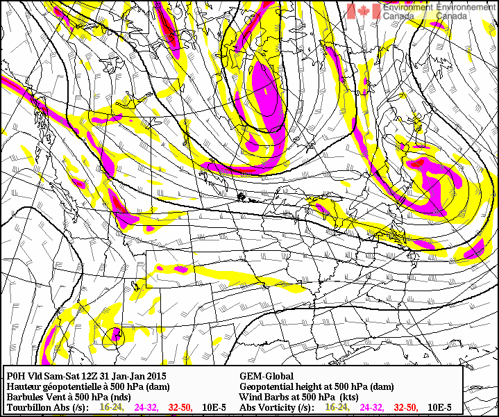
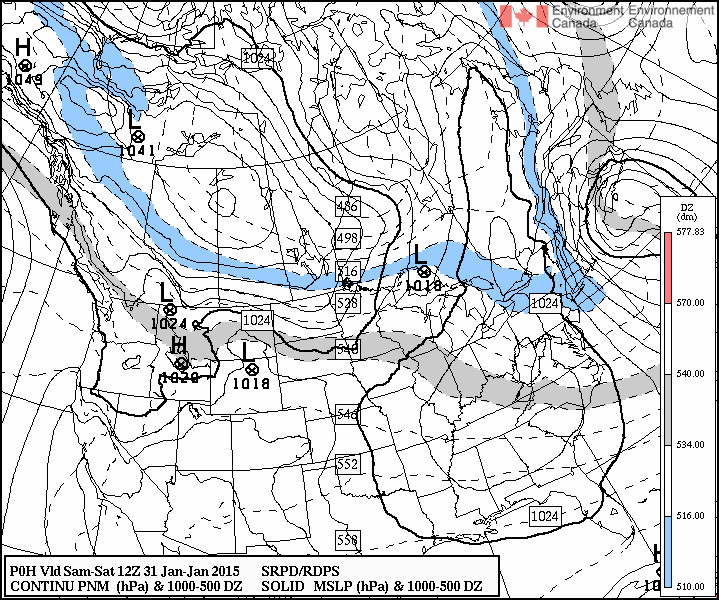
     • 500 hPa analysis for 12Z Saturday (and 0h GDPS prog). Firm WNW flow. Shortwave at Ab. Elbow. (as per forecasters' discussion)
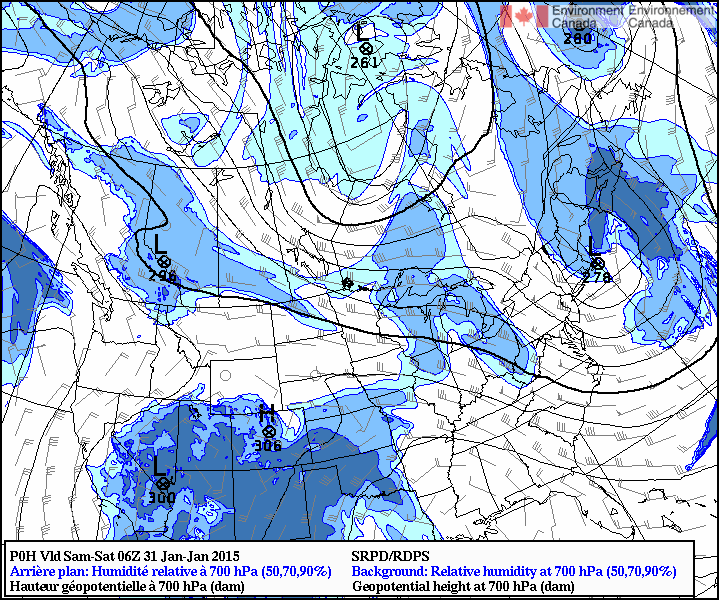
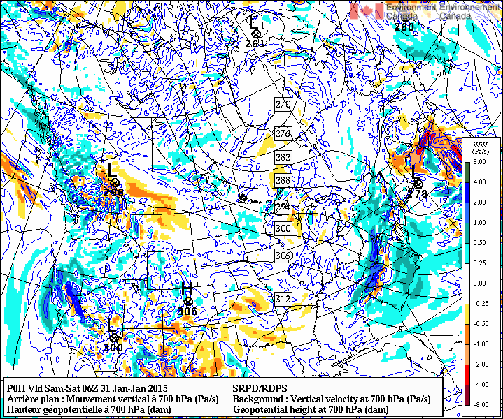
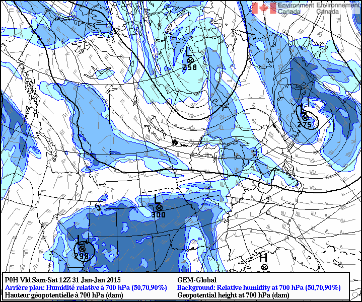
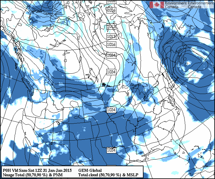
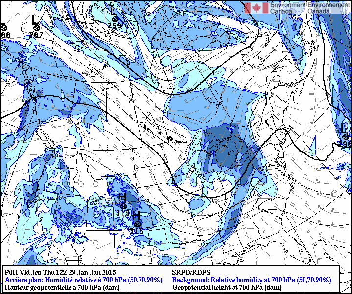
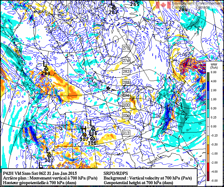
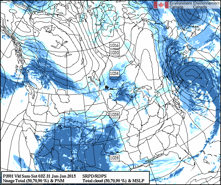
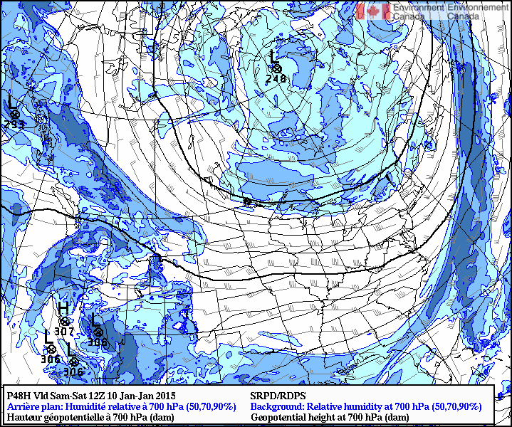
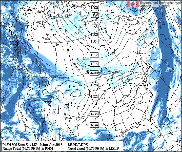
     • The RDPS 0h prog valid 06Z Saturday: 700 hPa and omega at 700 hPa. The GDPS 0h prog valid 12Z Saturday: 700 hPa and total cloud. We see the general flow pattern that had been predicted, and the humidity and cloud aloft. The closed upper low (seen in the 06Z analysis) didn't amount to anything significant.
     • The 12Z 700 hPa analysis
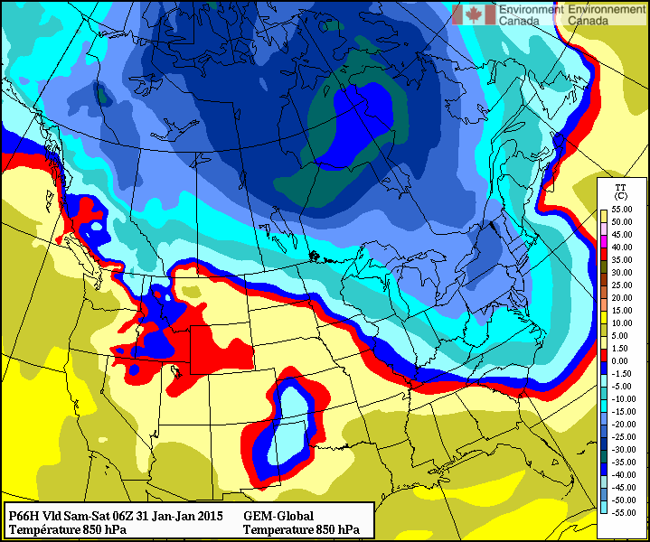
     • The 850 hPa analysis indicates fairly uniform temperature at that level over C. Alberta
     • Edmonton hourly weather to 07 MST Saturday.
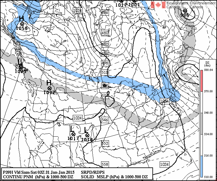
     • The RDPS 0h prog valid 12Z Saturday: MSLP & thickness shows the thickness to be a few dam colder than JDW's forecast (of 516 dam)
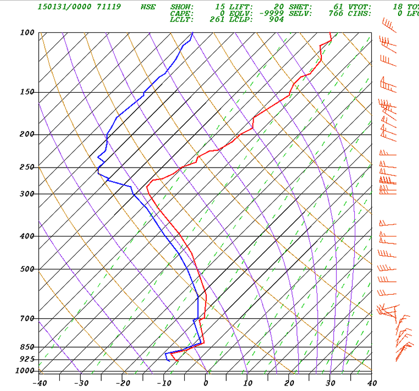
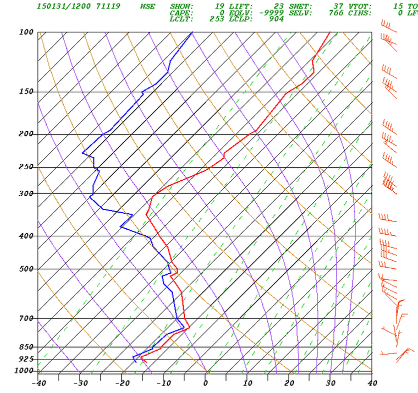
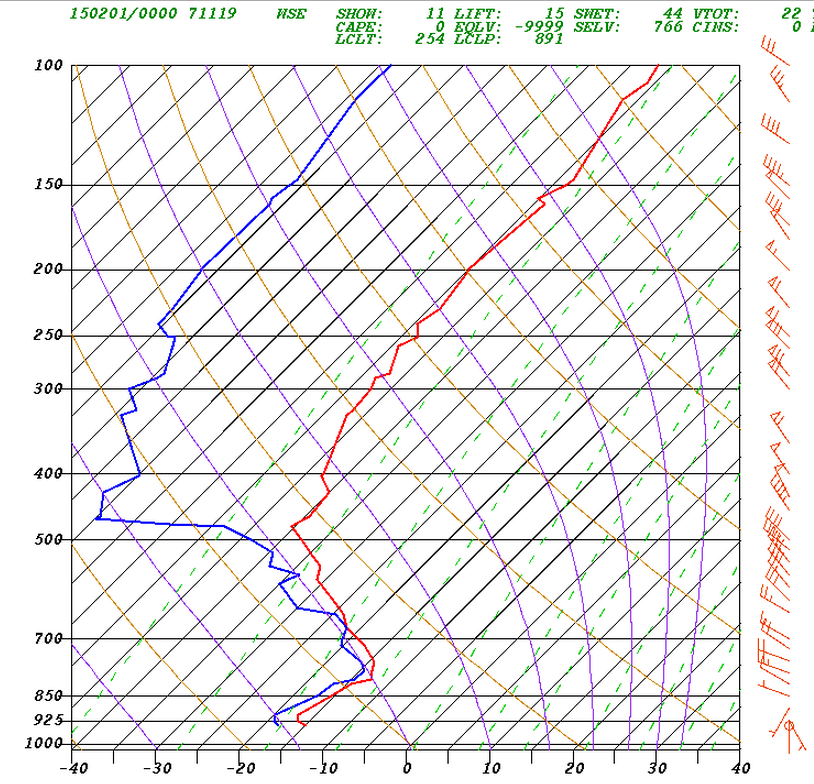
     • Stony Plain soundings for 00Z and 12Z Saturday 31st and for 00Z Sunday 1 Feb. Especially at 00Z Saturday we see the cold, low level air moving south beneath the westerly current aloft. By 00Z Sunday it would appear the tropopause has dropped to about the 500 hPa level!
     • CYEG Metars. Mix of cloud types, incl. middle cumuliform at low and mid levels.
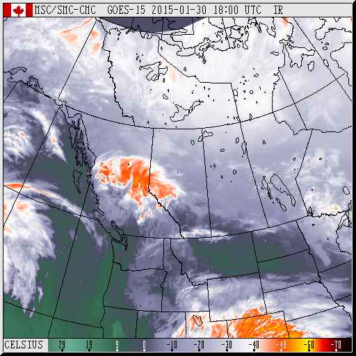
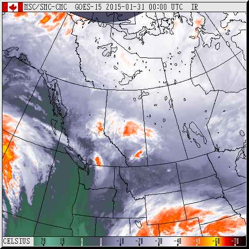
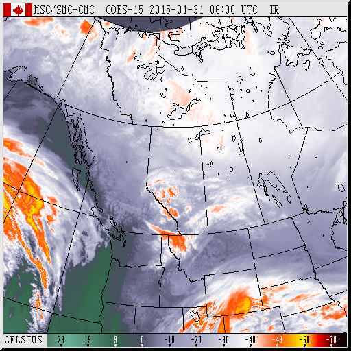
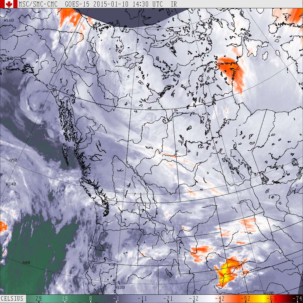
     • GOES IR 18Z Fri, 00Z Sat, 06Z Sat. Doesn't tell us anything very specific, except the timeing and location of high cloud tops.

• Thurs. 29 Jan. Isobaric coordinate system: vertical velocity (omega), material derivative, continuity equation, momentum equations, geostrophic wind. Link between horizontal divergence and ascent. Thermal wind. Summary of the geostrophic paradigm for weather evolution.

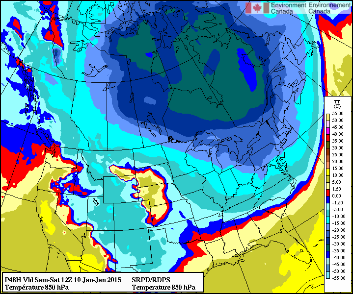
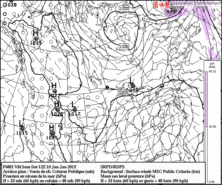
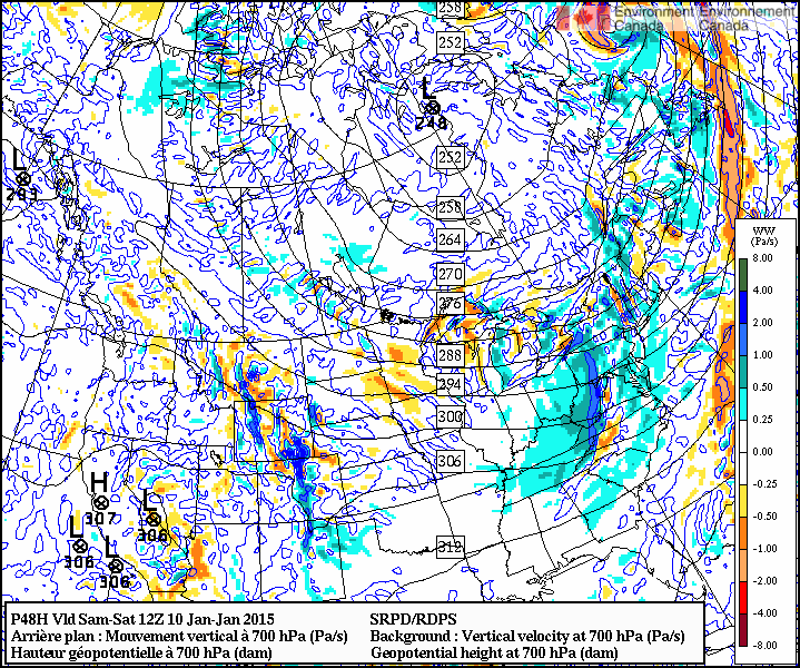
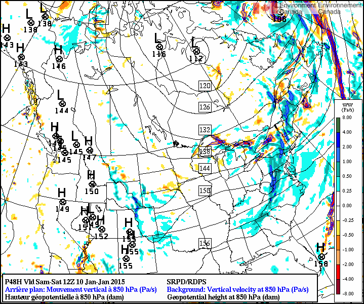
  Exercise: Prepare and document your forecast for C. Alberta for Friday and Saturday.

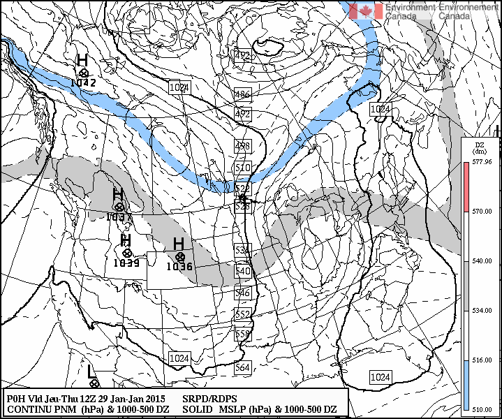
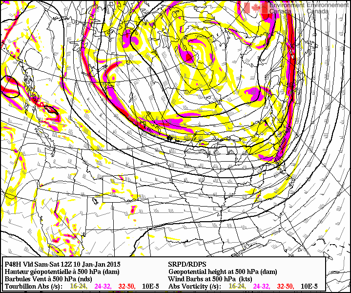
  JDW's forecast, based mostly on the evidence archived below (i.e. progs initialized at 12Z today) as well as other charts briefly perused (such as 500 hPa height/vorticity):

  • RDPS MSLP and thickness as of 03Z Saturday: some 9^oC of cooling compared with 12Z today
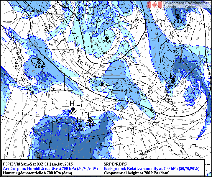
  • RDPS 700 hPa pattern as of 03Z Saturday, compared with 12Z today. A weak upper low, plenty of humidity aloft, orientation of the flow aloft turning from W to NW. [Notice that the 700 hPa wind will be blowing over the top of a cold, southward-moving surface current]
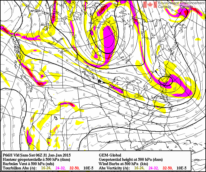
  • GDPS 500 hPa pattern as of 06Z Saturday: firm WNW flow (no danger of long residence times overhead, whatever comes); a shortwave to pass south of C. Alberta
  • GDPS 850 hPa thermal pattern as of 06Z Saturday: notable NS gradient, colder air invading
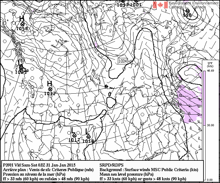
  • RDPS surface wind 03Z Saturday (outflow from the arctic high)
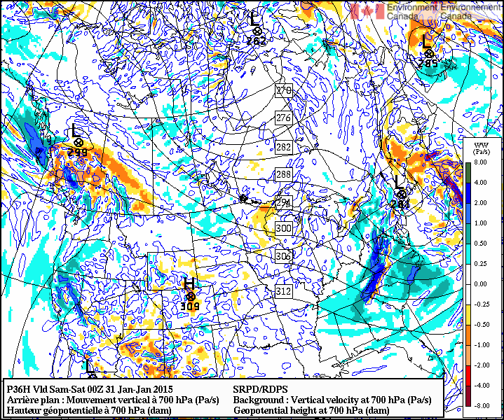
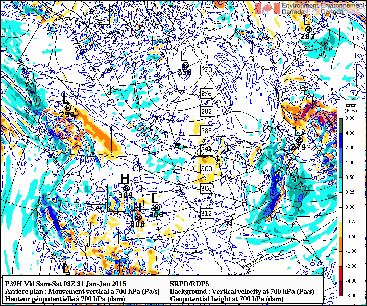
  • RDPS omega at 700 hPa as of 00Z Saturday (03Z, 06Z). Plenty of synoptic scale ascent, up to about -1 Pa/s which is roughly a 10 cm/s updraft: very useful for producing precipitation from the available moisture
  • RDPS total cloud as of 03Z Saturday (correlates with patterns of humidity, ascent and precip?)
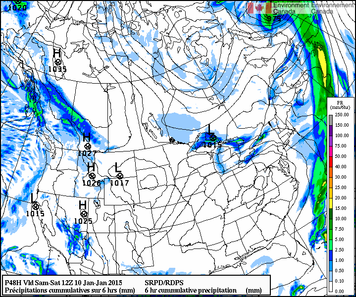
  • RDPS precip swath for 12 hrs prior to 12Z Saturday
  • NAM prog precip swath for 6 hrs prior to 06Z Saturday
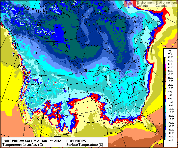
  • RDPS surface temperature for 12Z Saturday (puts us about -15^oC, agreeing with the meteogram below and only 5^oC colder than at 12Z today)
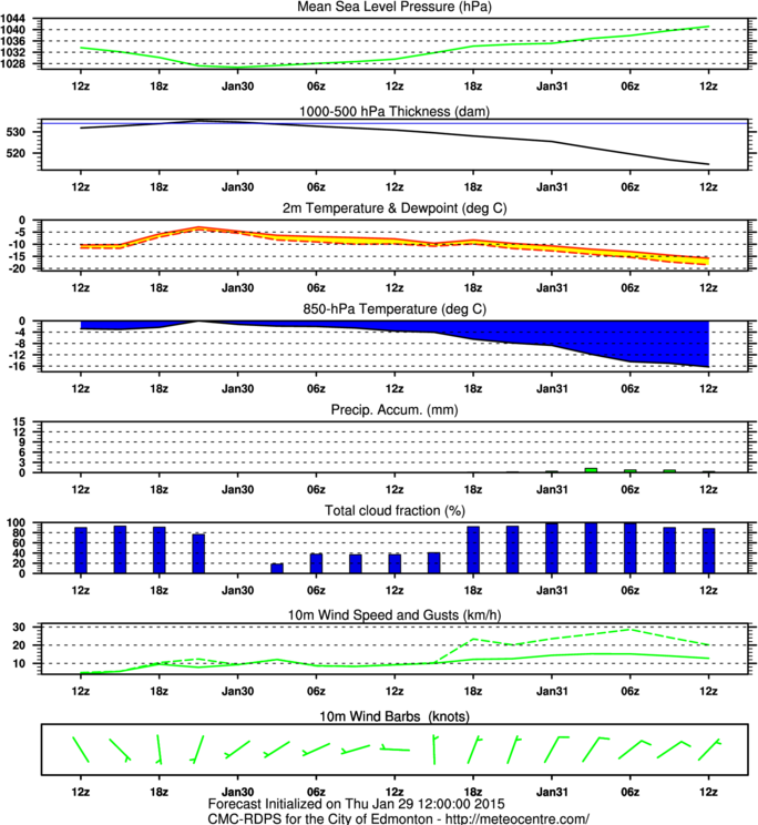
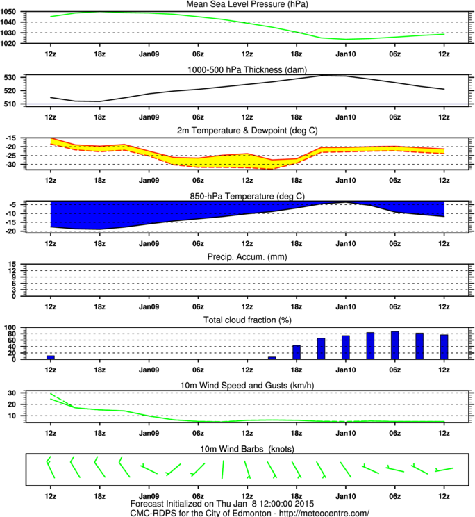
  • RDPS meteogram for Edmonton
  • Finally, is your forecast broadly consistent with the forecasters' discussion?
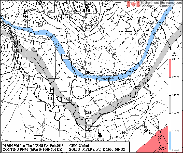
  According to the GDPS 156 h prog we get a fresh incursion of mild air by the middle of next week.

• Tues. 27 Jan. Quick update on the east coast storm (which we had spotted in the progs days earlier; here's a NY Times article that puts complaints about the forecasting in context). Starting with the 1st law dq=c_p dT - α dp (where α=1/ρ), derive (i) the adiabatic lapse rate and, (ii) Poisson's law defining potential temperature. Horizontal momentum equations in vector and scalar forms [Terminology: U=(u,v,w) and V=(u,v).]

  Exercises:

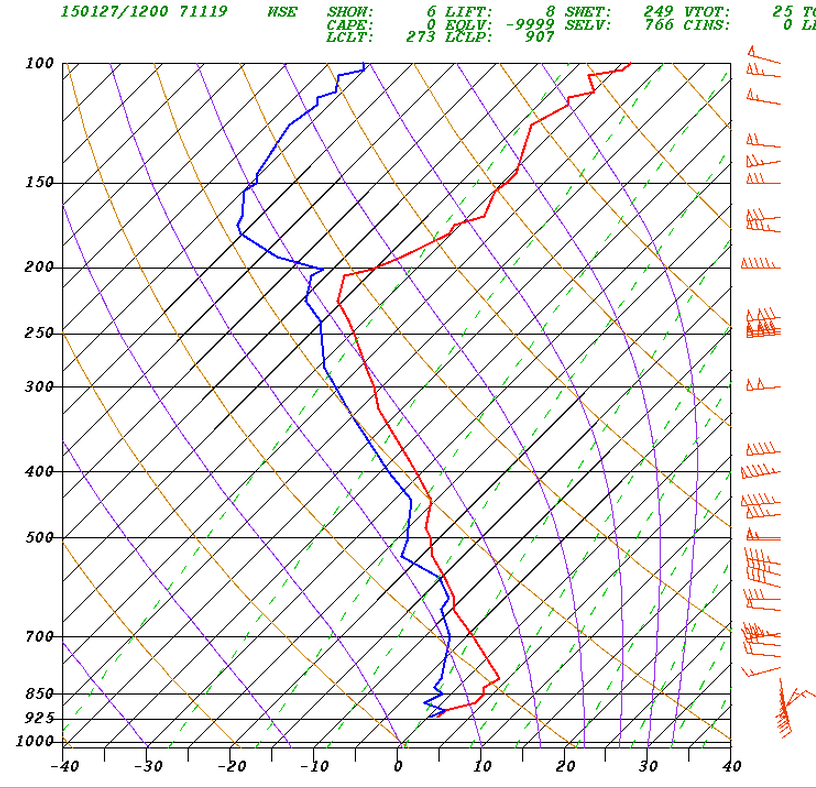
  1. Plot today's 12Z temperature soundings for Fort Nelson (YYE) and Stony Plain (WSE) on a blank Skew-T chart (colour pdf)

     Answer:

     • Fort Nelson (YYE) skew-T (and YYE data)
     • Stony Plain (WSE) skew-T (and WSE data)

  2. Perform the following "back-of-the-envelope" calculations, making whatever simplications might simplify the task. Suppose the 974-865 hPa layer on the Fort Nelson (YYE) sounding were considered (as a simplifying approximation) to be isothermal, with T=-20^oC. How much energy (per unit ground area, J m^-2) would be required to raise its temperature isobarically (i.e. dq [J kg^-1] =c_pdT ) to -10^oC? If this were to be supplied by way of a positive surface sensible heat flux Q_H=100 [W m^-2], how long (t) would this flux have to operate to achieve the stated adjustment? If, alternatively, the adjustment were to be achieved by condensing water vapour [L_v ≈ 2.5x10⁶ J kg^-1], what mass of water vapour per unit ground area would need to be condensed? And if all this mass fell as precipitation, what would be the accumulated depth of (liquid) water?

     Here is the NCEP 6h forecast for the surface sensible heat flux density (field of Q_H) valid 18Z today... (from here). A speculation: the model's band of positive (green) heat flux across NE BC and N Alberta signals cold surface air moving south out of the arctic high over (relatively) warm ground. This is plausible because the surface heat flux is invariably modelled by the bulk aerodynamic method

     Q_H = α ρ c_pU₁ (T_sfc - T₁ ),

     where U₁, T₁ are model wind speed and temperature at the lowest atmospheric level, T_sfc is the temperature of the underlying surface, ρ & c_p have their usual meaning, and α is a calibrated constant. [This is essentially the textbook's Eq 1.59, however the latter gives the kinematic heat flux.]

     Answer: the question is motivated by the appearance, on the sounding, of a layer of cold air underneath a sharp inversion aloft. How much mass (per unit ground area) lies in the column between 974 and 865 hPa? The thickness of the layer is Δz=1261 - 381 m = 880 m. Density at the lower level is ρ=97400/(287 * (273-19))= 1.3 kg m^-3 (it would have been OK in the present context to have simply guessed a reasonable value for ρ). Multiplying we have ρ Δz = 1144 kg m^-2. Then the energy required per unit ground area to warm this layer by 10^oC is E=1144 x 1000 x 10 = 1.1 x 10⁷ J m^-2.

     If the needed energy were supplied at a rate of 100 [W m^-2] the warming process would take t=1.1 x 10⁵ sec or roughly 30 hours.

     If it were supplied by condensing water vapour (L_v=2.5 x 10⁶ J kg^-1), one would need to condense about 4 kg m^-2. Four kg of water has a volume of 0.004 m³ to the depth of the condensed water would be 4 mm.

• Thurs. 22 Jan. Representation of the rate of thermal advection in coordinate-independent form, in the conventional local Cartesian coordinate system, and in the natural coordinate system. Fick's law for the total mass flux density of any component of a mixture, and the formal statement of mass conservation.

  Let ρ_A and n_A be the volumetric mass content ("density") and the mass flux density of a component "A" in a mixture A+B whose total density is ρ=ρ_A+ρ_B (in the meteorological context, typically A may represent water vapour, and B "dry air"). Then Fick's Law may be written

  n_A = u ρ_A - ρ D_AB ∇ (ρ_A/ρ)

  where u is the bulk velocity vector ("wind"). Thus the first term is the convective part of the mass flux density, the second the diffusive part. The molecular diffusivity has the unit [m² s^-2], and D_AB=D_BA.

  By the same steps as we took to get a conservation eqn for heat, the conservation equation for "A" is

  ∂ρ_A/∂t = - ∇ • n_A + S_A,

  and a more specific law is obtained by substituting Fick's law for n_A. Now let "A" be the "air," for which there is no source term. Furthermore "air" cannot diffuse in "air", so there is no diffusive contribution to the mass flux of "air." Then the conservation equation, given the special name "continuity equation", reads:

  ∂ρ/∂t = - ∇ • (ρ u).

  Exercises:

  1. Compute the geostrophic wind speed at 500 hPa over Edmonton (12Z Thurs. 22 Jan.) Answer: |V_g|=(g/ f) ΔZ/Δ n ≈ 23 m s^-1 (where f=1.17 x 10^-4 s^-1)
  2. Using the wind speed reported by the radiosonde, compute the advective rate of change of temperature at the 850 hPa level over Churchill, Manitoba (12Z Thurs. 22 Jan.) Answer: A_T = - |V_g| ΔT/Δ s ≈ (-17.5) x (-5/1.6E5) x 3600 ≈ 2 K hr^-1.
  3. Compute the geostrophic wind speed and the implied advective rate of change of temperature at the 850 hPa level over Winnipeg (12Z Thurs. 22 Jan.) Answer: with f≈ 1.11 x 10^-4 s^-1 (roughly 50^oN), one finds |V_g| ≈ 22 m s^-1 and A_T ≈ 2 K hr^-1.
  4. Based on NCEP's GFS prog, broadly summarize the weather to be expected along the U.S. eastern seaboard and in maritime eastern Canada for the next two weeks. Choosing (say) New York City or St. John's Newfoundland, on which day(s) during the forecast period are surface winds liable to peak? [A sequence of strong storms were forecast to move up the east coast.]

  Comment on exercises 1-3: These calculations are very approximate, leaving choices to your discretion: which pair of contours to take?, how much to fret over irregularities in their spacing? Two significant digits is plenty.

• Tues. 20 Jan. Heat flux density vector in the case that heat transfer occurs by convection alone, viz. Q= ρc u T where u is the velocity vector; or by both convection AND conduction, Q= ρc u T - ρc κ ∇ T. Consequent form of the equation expressing conservation of heat (emergence of the temperature "advection" term from the divergence of the convective heat flux).

  Exercises:

  1. Complete the exercise of previous class
  2. Choose an equatorial sounding and a polar sounding. For each of these, compute the virtual temperature T_v = T[1 + 0.61 q] at the 850 hPa level ("P"), and compare it with T. Note: in this formula the specific humidity q is in [kg/kg]. To get q:
     • obtain the vapour pressure e from the given dewpoint using the equilibrium vapour pressure table (here for sub-zero temperatures the equilibrium value is computed with respect to ice).
     • as a cross check , compute RH and compare with the value given on the sounding (this should clarify for us whether RH had been calculated using equilib. v.p. over ice or liquid: Conclusion, the soundings give RH with e* evaluated over water, even for sub-zero temperatures)
     • then q=0.622 e/p

     Example, Acapulco (12Z Jan. 20, 2015). At 850 hPa e=*(T_d)=1468 Pa, q=1.07E-2 [kg/kg] and T_v = 291.44 whereas T=289.55K... thus T-T_v=1.89 K. RH=79%.

     Example, Resolute (12Z Jan. 20, 2015). At 850 hPa, and if we use the svp over ice we get e=*(T_d)=48.6 Pa and *(T)=67.8 Pa implying RH=71.7%... but the tabulation on the sounding gives 74%. If one uses the formula by Buck (1981), then e=*(T_d)=0.6353 hPa and *(T)=0.8585 hPa implying RH=74%. Carrying on, q=4.65E-4 [kg/kg] and T_v = 248.92 whereas T=248.85K... thus T-T_v=0.07 K. Similar results follow if one uses the Goff-Gratch formula for s.v.p. with respect to liquid water.

  3. From this morning's CMC 850 hPa and 700 hPa analyses, and focusing on the Edmonton region:
     • compute the potential temperature θ for each level. [Use Poisson's Law, Eq 1.24, taking ground-level pressure as reference, p₀]
     • compute the relative humidity RH and the absolute humidity ρ_v for each level. [From T, T_d you will need to compute the actual vapour pressure e = e_*(T_d) and the equilibrium vapour pressure e_*(T) using a table.]
     Compare your calculations with values given on the Stony Plain sounding.

     Answer: Surface pressure at Stony Plain was 930 hPa. Then θ₈₅₀=(273.15-5)*(930/850)^0.287 ≈ 275.16 K = 2.01^oC. Similarly, θ₇₀₀ ≈ 281.17 K = 8.02^oC. These values differ greatly from the tabulated "THTA" on the sounding, because values on the sounding use different reference pressure. Note however that they concur with values used by following a dry adiabat on the sounding, from (P,T) to the surface.

• Thurs. 15 Jan. Overview of present weather (focus, W. Canada). Theory: Developing an intuition for the transport equations of Meteorology/Fluid Mechanics: derivation of a general heat budget equation

  ρc ∂T/∂t = - ∇ • Q + S,

  where ρ is the density and c the specific heat capacity of the medium, Q is the (vector) sensible heat flux density and ∇ • Q ≡ div Q its divergence, and S is the volumetric production rate; Fourier law Q= - ρc κ ∇ T for the heat flux density due to conduction (alone), κ [m² s^-1] being the thermal diffusivity; deducing the meaning of the "heat equation."

  Exercises

  1. Based on the Stony Plain (wse) sounding data (12Z Wed. 14 Jan.; here's the skewT diagram), and neglecting the effect of water vapour on density:
     • compute an effective mean density for the 924-919 hPa layer, using the hydrostatic equation [ρ=1.19 kg m^-3]
     • compute the actual densities at 924 hPa and 919 hPa levels, using the ideal gas law [ρ=1.18, 1.19 kg m^-3]
     • compute the mean temperature of the 924-919 hPa layer according to the hypsometric equation [T=270.88 K = -2.26 ^oC. This is in poor agreement with the observed temperatures, possibly reflecting observational error of the rapidly ascending sonde?]
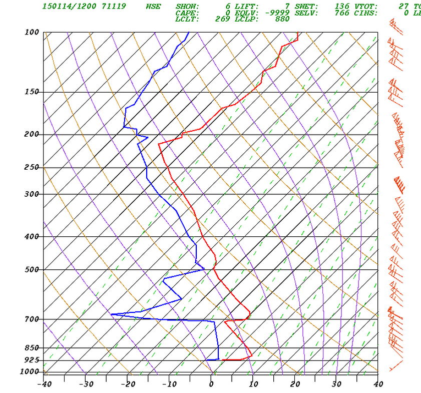
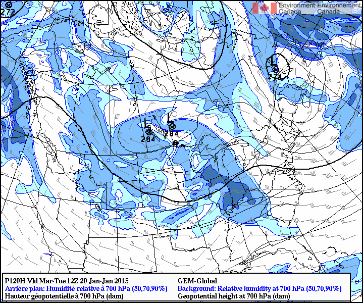
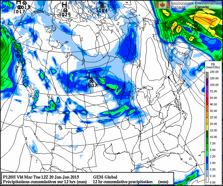
  2. Prepare your own forecast for the weather in (your choice) Edmonton or Winnipeg at around 12Z on Tuesday 20 Jan. [We ran out of time on this.]

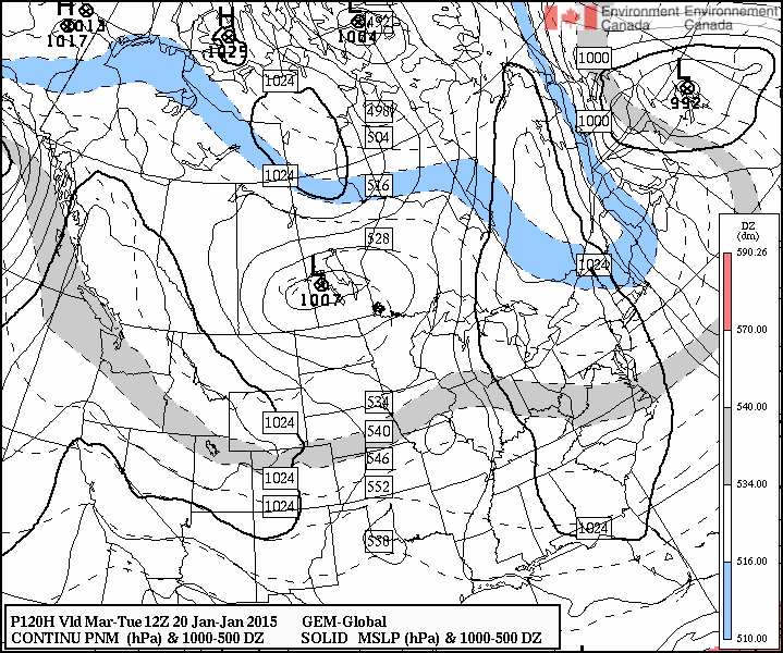
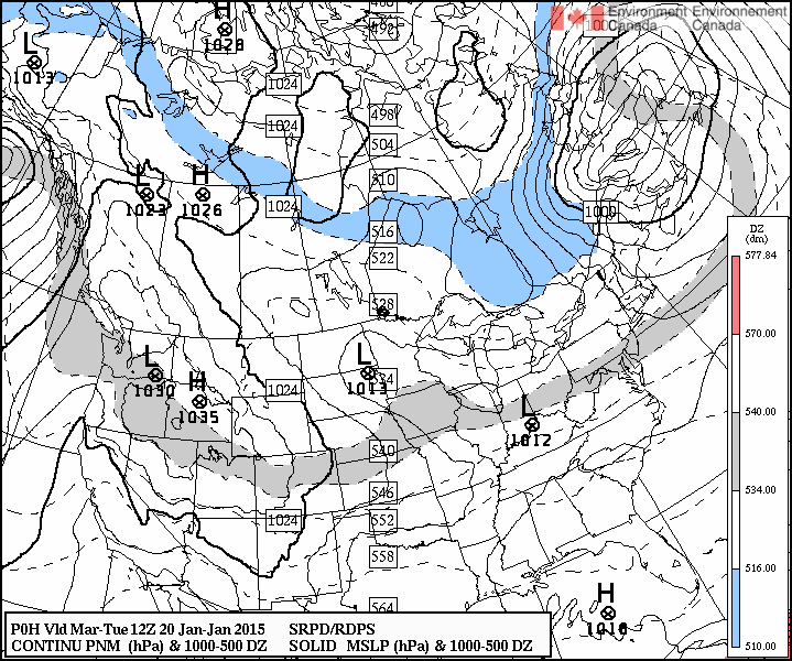
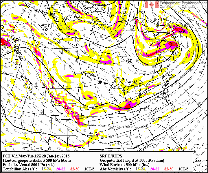
     JDW's take from the 120h GDPS prog initialized at 12Z today (Thurs. 15) and valid 12Z Tuesday 20 Jan., focusing on S. Manitoba:

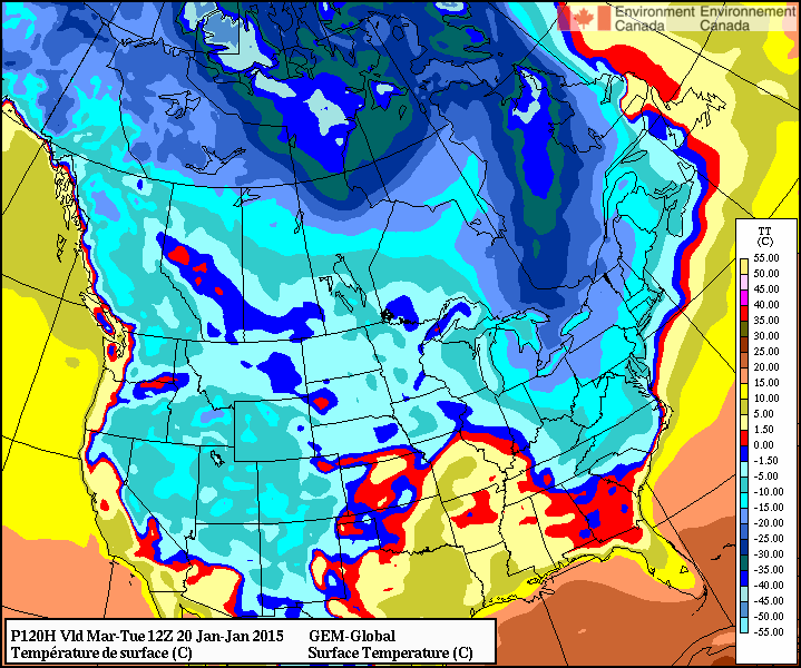
     • a low over S. Manitoba shows up in the MSLP panel (thickness about 528 dam, by no means extremely cold; this is confirmed by the Tsfc panel). The low is well defined, but not particularly deep.
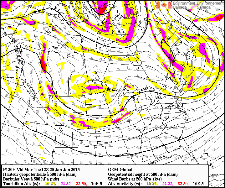
     • the low is "vertically stacked," i.e. there's a closed upper low overhead at 500 hPa
     • plenty of moisture aloft over Winnipeg, see 700 hPa panel
     • snow is a distinct possibility, see 12h cumulative precip, but Winnnipeg might just contrive to be in a dry spot (warm sector?)
     Summing up: Next Tuesday Winnipeg will not be too cold, but it will be cloudy and windy. There is likely to be some snow (and blowing snow).

     Verification: The RDPS 0h prog for MSLP and thickness valid 12Z Tues 20 Jan. shows a NW-SE oriented trough through S. Saskatchewan (broadly, as foreseen) but the focused low of the 120h prog is not there. Thickness (528 dam) matches the forecast. The forecast closed low at 500 hPa over Winnipeg is absent, see the RDPS 0h prog for the 500 hPa level: note, however, that on close examination there is a vortex over the Dakotas, such that if contours had been plotted at a finer interval, we'd have seen a closed centre.

• Tues. 13 Jan. Review. Equations expressed in vector form are coordinate-system independent. The "grad operator" (∇), a coord.-system independent notation for the gradient; can operate on a scalar to produce a vector (∇a) or on a vector to produce a scalar (∇ ⋅ A). Form of the grad operator in a Cartesian coordinate system. The Laplacian (or "diffusion" or "curvature") operator (∇² ≡ ∇ ⋅ ∇), operating on a scalar. The heat equation; Fourier's law of conduction; threefold classification of terms in the transport equations: storage terms, transport terms, source/sink terms. Connection between Lagrangian ("material," or parcel following) time derivative D/Dt and the local tendency in time ∂/∂t. Definition of a "conserved" property. [Note: in the course of the lecture the symbol q was used as a generic field; Q featured twice, as the (kinematic) heat flux density as given by Fourier's Law; and as the label for "source/sink" terms in transport equations].

  Exercises (a follow-up from our forecasts of last Thursday):

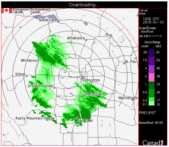
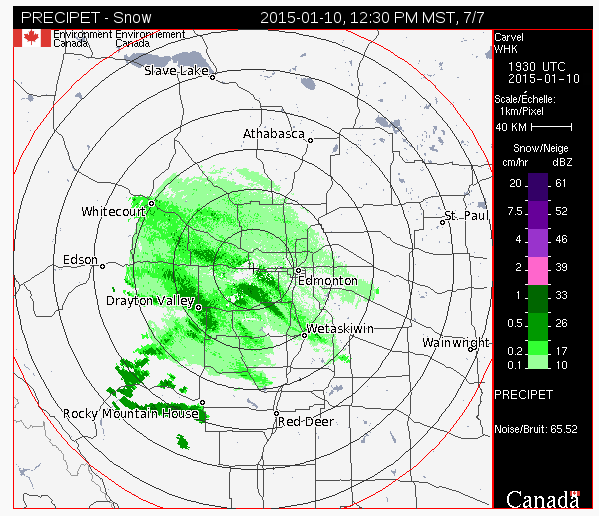
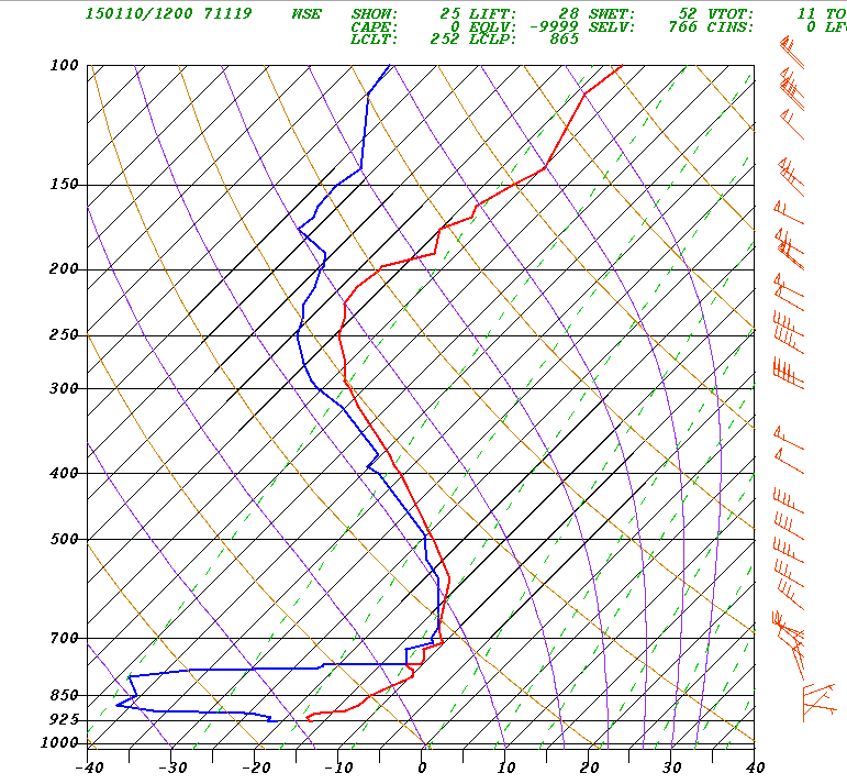
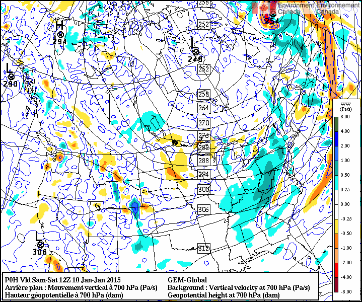
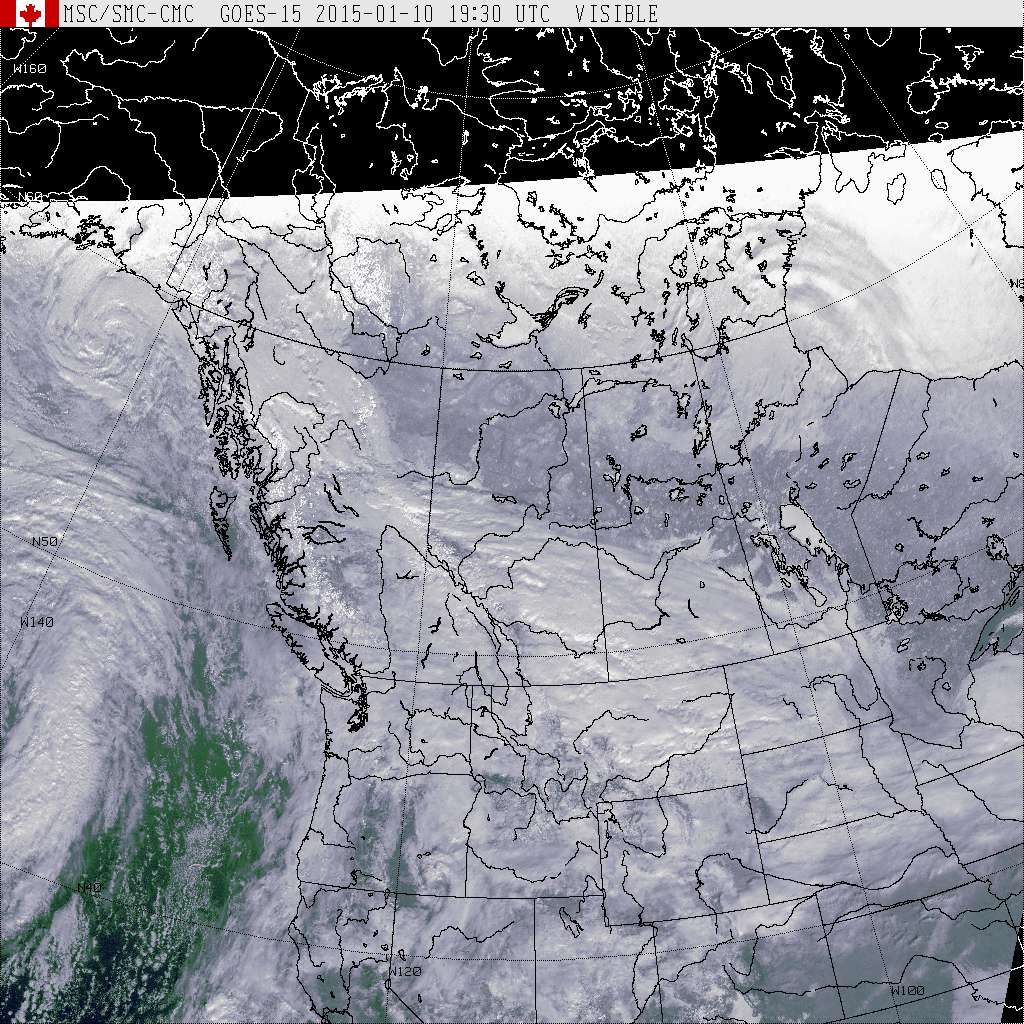
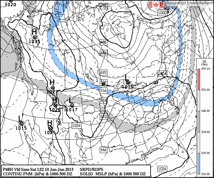
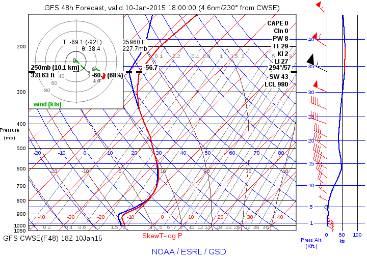
  • Peruse the maps/images below that depict C. Alberta meteorology on the morning of Saturday 10 Jan., and jot down your own inference as to the actual weather (a few paragraphs at most): each student will then relate what he/she noted to the class. (We concluded the overall flow configuration agreed with the forecast. The prolonged snowfall event had been perhaps the main surprise, certainly for JDW. Though less than 3 cm (liquid water equiv.) was reported, quite a bit of shovelling was called for. The sounding -- very stable -- featured quite dry air spanning from just above the surface to about 750 hPa, with saturated air above that. Surface wind was upslope, which may have contributed to the sustained snowfall. Weak ascent noted at 700 hPa on the synoptic scale, liable to have been a factor. Thickness, at 527 dam, a little milder than forecast.)
  • Swap your forecast from last Thursday for that of another student. Comment constructively on each others' forecasts.
    • Hourly weather for Edmonton City Center
    • Daily weather at YEG (Edmonton Int'l Airport)
    • Carvel radar plot 07:30 MST (14:30Z) and 12:30 MST
    • Stony Plain Skew-T diagram (12Z) and sounding data
    • Surface analysis (18Z)
    • 850 hPa analysis (12Z)
    • 700 hPa analysis (12Z)
    • Omega at 700 hPa (from the GDPS 0h prog, valid 12Z)
    • GOES ir image 14:30Z
    • GOES vis image 19:30Z
    • MSC forecasters' discussion 07CST
    • Public forecast for Edmonton as of 05 MST Saturday 10 Jan.
    • RDPS 0h prog valid 18Z (MSLP and thickness)

• Thurs. 8 Jan. Derivation of the hypsometric equation (c.f. Lackmann's Eq 1.37) as background for Assignment 1. Natural coordinate system. Expression for rate of thermal advection in the natural coordinate system. Quick update on changes in the meteo. since previous class.

  Exercises:

  • Prepare your own forecast for conditions in C. Alberta at 18Z Saturday 10 Jan. (Here is JDW's forecast, uploaded 13 Jan.)

    Archive of CMC's RDPS 48h progs (valid 12Z Saturday 10 Jan.), added after class:

    • MSLP & DZ (c.f. NAM 54h vld 18Z)
    • 700 hPa (c.f. NAM 54h vld 18Z)
    • Total cloud
    • Temperature at 850 hPa
    • Surface wind
    • Omega at 700 hPa
    • Omega at 850 hPa
    • 500 hPa height & vorticity (c.f. NAM 54h vld 18Z)
    • Cumulative precip (previous 6 hours)
    • Meteogram based on RDPS
    • Model sounding for (near) Stony Plain (GFS 48h prog)

  • Estimate the rate of thermal advection at YQD (The Pas, Manitoba) at the 850 hPa level, 12Z today (8 Jan.)... [Answer added 13 Jan.: advective cooling at a rate of ∼3 K hr^-1.]

• Tues. 6 Jan. Orientation to EAS 372. Course Outline. Grading. Scope. Familiarization with web weather resources. Discussion of present cold period, with attention to recognizing features mentioned by the forecasters (and how to find these charts).

Link to Earth & Atmospheric Sciences home page.

Last Modified: 17 Apr., 2015